The job-script file named "input.data" is needed to
execute MPDyn. Users should write the detailed simulation condition in this
file. Several dozens of keywords are available. Some keywords are essential and
should be written explicitly. Many parameters to be written in this file have
default values, which are used when no value is given. Script to set the keyword
should start with the line,
>> [KEYWORD]
and ends with the
line,
<<
The optional keywords should be given in the lines between
the above two lines. Any lines starting with the character '!' or '#' are
regarded as comments and ignored. If the line contains the character '!', any
words described after '!' are also regarded as comments. One can check if the
simulator interprets job scripts correctly by inserting the line,
CHECK
in
any place in this file. Then one obtains the file, "CHECK_INPUTS.(JOB_NAME)", in
which the options that the simulator interpreted are described.
In the
followings, dozens of keywords, including the optional keywords, are explained
in details.
Each simulation run is assigned a name, called "Job
name". If no name is declared, the default name,
JOB_YYYYMMDD_HHmm
is
assigned. Here
YYYY: year, MM:month, DD:day, HH:hour, mm:minite
The time
when the simulation started is referred.
| >>
JOB_NAME TEST_JOB << |
With this flag, user can select the directory to which this software generates the monitoring-data files during the MD runs. This monitoring files includes JOB_NAME.moni (thermodynamic data), JOB_NAME.r*** (trajectory data), JOB_NAME.v*** (velocity data), JOB_NAME.f*** (force data), JOB_NAME..Temp (DPD temperature), JOBNAME_Pres (DPD pressure), JOB_NAME.Ener (DPD energy), JOB_NAME.Vir (DPD virial), JOB_NAME.MSD (DPD mean square displacement), etc. When this flag is not given, the current working directory is used for this purpose.
| >>
DIR_NAME /scratch/MPDyn/ << |
In this case, this program generates e.g. a energy file, /scratch/MPDyn/(JOB_NAME).moni.
This flag is used to set the simulation method listed
below.
[ MD, HMC, PIMD, CMD, DPD, MM, NMA, Analysis ]
| MD | molecular dynamics |
| HMC | hybrid Monte Carlo |
| PIMD | path integral molecular dynamics |
| CMD | centroid molecular dynamics |
| DPD | dissipative particle dynamics |
| MM | Energy and force calculations for a configuration |
| DynaLib | MD library that can be called from QM simulators** |
| NMA | normal mode analysis |
| Analysis | analysis of stored molecular trajectories |
** In case of 'DynaLib', the keywords, "JOB_NAME", "SYSTEM", "PBC" or not, and 'TOTAL=' and 'CURRENT=' of "STEP_NUMBER" must be given to proceed molecular dynamics correctly.
| >>
METHOD MD << |
This flag is used for the selection of the force field
parameter set.
| FF= | The name of force filed | necessary |
| TOPFILE= | The name of topology file to be used | not necessary |
| PARFILE= | The name of parameter file to be used | not necessary |
| PSF= | PSF filename | only for CHARM |
As for "FF=" flag, available force fields are [CHARMM, OPLS,
EAM, BKS] for molecular simulations, [CG] for coarse-grained molecular
simulations, and [F11, F22, F23] for dissipative particle dynamics.
Fnm for DPD is to determine the functional form for nonbonded interaction
as
F(n)(m) :
Fc= a ( 1 - (r / rc)n )m
n,m = {1,1} is the choice of conventional functional form.
The CHARMM, OPLS, BKS, and CG force fileds require topology and parameter
files. Those filenames should be given using the flags of "TOPFILE="
and "PARFILE=", though not always needed. They have default names;
top_charmm27.prm and par_charmm27.prm for CHARMM, top_OPLS.prm and par_OPLS.prm
for OPLS, top_BKS.prm and par_BKS.prm for BKS, and top_CG.prm and par_CG.prm
for CG forcefields, respectively. When one uses rigid-body model, some
optional data are needed in the topology file. Example file for CHARMM
and OPLS are provided in the directory ./param as top_charmm27_RB.prm and
top_OPLS_RB.prm, respectively. Users can use their own topology and parameter
files. Note that these files should be written in the CHARMM style. An
exception is the CG force field. For the CG force field, ~/CGparam/top_CG.prm
and ~/CGparam/par_CG.prm are the default topology and parameter files to
be used, respectively.
In case
of DPD, using "PARMFILE=", users can specified the parameter file. No script
given for "PARMFILE", it is assumed "./param/interaction.param".
| >> FORCEFIELD FF= CHARMM PSF= ./param/SYSTEM.psf << |
The system to be simulated is set by this flag.
| SYSMOL= | The number of components in the system | integer |
| MOLNAME= | Molecular name [for each component] * | integer |
| MOLNUM= | The number of molecule [for each component] | integer |
| ATMNUM= | The number of atom per molecule [for each component] ** | integer |
* To treat a polymer, user should give a molecular name
with the prefix, "Poly".
** When a polymer molecule is described, user
should read this flag as the degree of polymerization (the number of monomer)
.
| >> SYSTEM SYSMOL= 5 MOLNAME= AQP1 DPPC TIP3 Na Cl MOLNUM= 1 94 4029 6 8 ATMNUM= 3377 130 3 1 1 << |
*In this example, the system is composed by 1 AQP1(membrane protein) molecule, 94 DPPC(lipid) molecules, 4,029 TIP3 water, 6 Na+(sodium ion), and 8 Cl-(chloride ion).
| >> SYSTEM SYSMOL= 1 MOLNAME= PolyPE MOLNUM= 20 ATMNUM= 100 << |
*In this example, the system consists of 20 polyethylene (polymerization grade is 100).
The status of the starting configuration is specified. To start from the initial configuration written in the CRD-file format, "Initial"; or to restart from the last configuration of the previous simulation run, "Restart". (Default : "Restart") User can choose the data format (ascii or binary) for the restart configuration file, "restart.dat", using the flag, "FORM=". Two parameters can be used for this flag; "formatted" (ascii) or "unformatted" (binary). The default value is "unformatted". MPDyn updates the restart file every 1000 MD steps automatically. The file, "restart.dat", is overwritten at the moment. If you want to change the timing to update the restart file, you can choose the timing with the flag "BACKUP="; BACKUP= 10000 means that the restart file will be overwritten every 10,000 steps. You can choose 0 for this. In this case, MPDyn does not generate "restart.dat" until the MD simulation ends. MPDyn also generate a PDB file, final.pdb, at the same timing for restart.data if you put "PDB= ON" in this keyword. MPDyn generate "final.pdb" for the configuration of the last step of MD in any case. The PDB flag is used just to have a snapshot during MD calculations.
| >>
STATUS Initial FORM= formatted BACKUP= 10000 PDB= ON << |
The flag is a declaration that periodic boundary condition is used. If no description for this keyword free boundary is selected as a default. This option is valid only for molecular simulations.
| RC= | Cutoff lenth1 | real | default 12[Å] |
| RBOOK= | List-up length for book-keeping | real | default 14[Å] |
| RSKIN= | (can be used instead of RBOOK)2 | real | default 2[Å] |
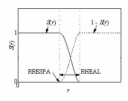
| RRESPA= | Distance for RESPA (CG model only)3 | real | default 6[Å] |
| RHEAL= | Heal region between Ffast and Fslow (CG model only)6 | real | default 4[Å] |
| MAXPAIR= | Maximum number of pair-list | integer | default 1,000,000 |
| TBOOK= | Interval for renewal of the book | integer | default 1 |
| VDWSWITCH= | Smooth switching off of vdW [ON/OFF]4 | default (depending on forcefield) | |
| VDWCORRECT= | Cut-off corrections [ON/OFF]5 | default ON |
1 RC= usually defines the cutoff length of LJ and Coulomb interactions (Ewald real-space term) except CG model is chosen in the FORCEFILED section. In case of CG model, RC= is used just to define the real space cutoff for the Ewald sum of the Coulomb interaction.
2 RBOOK = (RC+RSKIN) ; RSKIN is an optional flag and can be used instead of RBOOK. RSKIN is useful in case of CG model, because each pair of atoms can have different RC value. Neither RBOOK nor RSKIN defined, RSKIN=2 is used in the calculation.
3 RRESPA= is useful only when multiple-time-step algorithm is used. The value given here defines the short-range force, which updated with the stepsize of Δtmiddle. See TIMESTEP. The long-range force is updated with the stepsize of Δtlong. This flag is valid only when the CG model is used.
4 When VDWSWITCH= is 'ON', a smooth switching function is applied to the van der Waals (nonbond) interaction. (in the range of RCUTOFF-2[Å] to RCUTOFF). When this is 'OFF', the nonbond interaction is cut-off at the distance RCUTOFF, while the correction of energy and virial terms are taken into account instead. If the CHARMM force field is chosen, the default value is set to 'ON', otherwise 'OFF'.
5 The cut-off corrections for energy and virial are taken into account in their calculations when VDWCORRECT= 'ON'. However, when the tepering cut-off is selected (VDWSWITCH= 'ON'), this option is automatically inactivated. The choice of this option often affects the calculated pressure (or volume in the NPT ensemble) significantly. Usually 'ON' should be selected (default).
6 RHEAL= is useful only when
multiple-time-step algorithm is used. The value defines the range of the smooth
switching function applied for F(r); nonbond force, and Ffast and
Fslow are defined in the following manner:
Ffast = S(r)
F(r)
Fslow = [1 - S(r)]F(r)
| 1, r < a | |
| S(r) = | 1+y(r)^2*(2*y(r)-3), a < r < b |
| 0, for r > b |
where y(r) = (r^2 - a^2) / (b^2 - a^2), and a = RRESPA, and b = RRESPA+RHEAL.
| >> PBC RC= 10. RBOOK= 12. TBOOK= 15 << |
* In this case, since MAXPAIR is not defined explicitly, it is set to be the default value, 1,000,000.
Energy minimization is carried out, when this flag is written. As a default, it is invalid.
| METHOD= | Energy minimizing scheme | - | default SD( steepest descent) |
| ITERATION= | The number of iteration steps | integer | default 300 |
| DR= | The translocation distance per step | real | default 0.1 [Å] |
| ERROR= | The threshold of the convergence (relative error) | real | default 0.00001 |
| >> ENERGYMIN << |
The method to estimate the Coulomb interaction is described using this flag.
| METHOD= | [EWALD(default), PME, Cutoff, SCREEN] |
In case of EWALD, the following two flags are also valid.
| ALPHA= | α | real | default: 0.238 [Å-1] |
| K2MAX= | k2max | integer | default 81 |
In case of PME (particle mesh Ewald), the following flags are valid.
| ALPHA= | α | real | default: 0.238 [Å-1] |
| NGRIDX= | grid size along x-axis | integer | default 32 [-] |
| NGRIDY= | grid size along y-axis | integer | default 32 [-] |
| NGRIDZ= | grid size along z-axis | integer | default 32 [-] |
| ORDER= | The order of B-spline interpolation | integer | default 4 [-] |
SCREEN option is available only when "Coarse-grained
(CG)" force field is used. This is a default value for the "CG" force field,
assuming κ, r0, and relative permittivity, εr are 0.5, 0
and 1, respectively.
screening Coulomb : U =
c*qi*qj/(r*εr)*exp(-κ(r-r0))
; c =
1/(4*π*ε0)
These parameters are changed using the following
flags.
| KAPPA= | κ | real | default: 0.5 [-] |
| RSHFT= | r0 | real | default: 0.0 [-] |
| EPS_R= | relative permittivity | rea; | default 1 [-] |
| >>
COULOMB METHOD= EWALD ALPHA= 0.250 K2MAX= EWALD << |
This flag is valid only if PBC flag is selected in case of all-atom MD/MC.
This flag sets the number of steps of simulations.
| TOTAL= | Total number of steps | integer | default 10000 |
| ENERGY= | Interval for storing energy | integer | default 1 |
| COORD= | Interval for storing coordinate | integer | default 10 |
| VELO= | Interval for storing velocity | integer | default 10 |
| CURRENT= | Current MD step (only for 'DynaLib') | integer | default - |
| ENE_AVE= | Averaged energy* [ON / OFF] | - | default: OFF |
| >>
STEP_NUMBER TOTAL= 1000000 ENERGY= 10 COORD= 20 VELO= 1000001 << |
* "ENE_AVE= ON" means that you get an averaged thermodynamic quantities for every certain steps defined by "ENERGY=" option, in an energy file, (Jobname).moni. Otherwise, you usually find an instanteneous values in the file.
This flag is used to fix the selected atoms to the specific position. The reference configuration is needed for this flag, so that "FILE=" subflag denotes the file name storing the reference configuration. If the filename is not specified, the initial configuration is used as the reference. There are two types of constraint method; "MASS": large mass, and "HAM": harmonic constraint. For the last case, one can regulate the spring constant, k, with the line starting from "k=". Unless specified, the default value of k, 100kcal/mol, is used. There are several ways of specification of the atoms to be applied the constraint. The keyword "COMPONENT" specifies the component number to be fixed. The constraint can be applied atom by atom in such a way that specifying the atom number. In case of protein molecules, the keywords, "COMPONENT_MAIN" and "COMPONENT_SIDE" are valid to select the main and side chains of the protein, respectively.
| FILE= | the filename of the reference configuration | - | default (initial.crd) |
| MASS [region] | The atoms are treated to have huge inertia | real | - |
| HAM [region] | Harmonic constraint | real | - |
| k= | The spring constant [kcal/mol] | real | default: 100.0 |
The constraint atom can be selected in the following ways;
| COMPONENT (component number) |
| COMPONENT_MAIN (component number) *protein |
| COMPONENT_SIDE (component number) *protein |
| (atom number i) (atom number j) ! Atoms numbering from i to j |
| >> FIXEDATOM FILE= ./param/RIni.data k= 1.0 HAM COMPONENT 1 HAM 736 1056 << |
*In this example, the molecules tagged component number 1 and the atoms numbering 736-1056 are fixed by a harmonic constraint with the spring constant, 1kcal/mol, to the reference configuration described in the file, "./param/RIni.data".
This flag is useful when a harmonic constraint of the center of mass (COM)
of a (group of) molecule(s) at a specific location. User can specify the
target group in two ways;
COMPONENT (component number) [coordinate: (x y z)]
( atom number - atom number) [coordinate: (x y z)]
| k= | The spring constant [kcal/mol] | real | default: 100.0 |
| >> FIXEDCOM k= 10. COMPONENT 1 (0. 0. 0.) (100-200) (10. 0. 0.) << |
This flag provides a way to apply the additional harmonic
constraint on the atom on a plane. User should describe the atoms, the spring
constant, the distance in a line.
(Atom i (integer)) (Atom j (integer))
(spring constant (real) [kcal/mol]) (distance (real) [A])
| >> OPTIONALBOND 1 5 2.0 2.5 7 12 2.0 2.2 15 22 2.0 3.0 << |
This flag provides a way to apply an additonal constraint for a dihedral
angle of the selected 1-2-3-4 pairs of atoms.
(Atom i (integer)) (Atom j (integer)) (Atom k (integer)) (Atom l (integer))
(spring constant (real) [kcal/mol/rad2]) (angle (real) [degree])
| >> FIXEDDIHEDRAL 1 2 3 4 100. 20. << |
This flag provides a way to apply the additional
constraint between arbitrary chosen pairs of atoms.
| AXIS= | Define the plane normal [X/Y/Z] | - | - |
The atom numbers, the spring constant, the location
(coordinate) should be given in a line.
(Atom number (integer)) (spring
constant (real) [kcal/mol]) (coordinate (real) [A])
| >> FIXONPLANE AXIS= Z 1 2.0 2.5 7 2.0 2.5 15 2.0 2.5 << |
In this case, three atoms (numbered 1, 7, and 15) are fixed on z=2.5 with a harmonic potential (k=2.0kcal/mol).
The number of steps to store the configurations in a file can be specified with this flag. The default value is 1000.
| COORD= | The number of steps | integer | default 1000 |
| VELO= | The number of steps | integer | default 1000 |
| >> DATA_PER_FILE COORD= 10000 VELO= 10000 << |
The data format of the configuration file is selected by this flag. There are three formats to be used for MD; ["formatted"(XYZ format), "unformatted", "DCD"(dcd format; NAMD standard)]. The "unformatted" is selected as the default.
| FORM= [FORM] | default: unformatted |
| >>
DATA_FORM_TRJ FORM= formatted << |
In addition, just for the analysis with molfile libraries using "MPDynS_MOLFILE", there are two more options for this format. TRR and XTC; both of which are GROMACS trajectory files.
This keyword is used to switch the standard output. Three options are available : OFF (default), ON (instantaneous energy etc.), DETAIL (debug; for developper)
| >>
STDOUT ON << |
During the simulation runs, this software generates (JOB_NAME).moni, which includes instantaneous thermodynamic quantites. This keyword has two values : ON(default) or OFF. If it's ON, the software also generates (JOB_NAME).ave, which contains the averaged thermodynamic quantities. The average is taken for each time interval of the output. This is NOT the accumulative average.
| >>
AVEMONITOR OFF << |
The flag is used to control the system pressure to a set point. Four types of barostat are available; AN: The Andersen barostat, A3 and A2: the Parrinello-Rahman barostat with the rectangular cell, PR: the Parrinello-Rahman barostat with the fully flexible cell, and ST: generalized stress control with the fully flexible cell. The difference between A3 and A2 is the number of degrees of freedom of the basic cell. A3 allows three cell lengths to fluctuate independently, though A2 apply a constraint between two of three cell edges. When A2 is selected, ISOPAIR option also should be given to specify the two cell edges to be coupled in their dynamics. If ISOPAIR= XY is chosen, for example, the simulation box fluctuate isotropically in x-y plane, but Lzz fluctuates independently.
| METHOD= | barostat type [ AN, A3, A2, PR, ST] | - | - |
| PEXT= | External pressure (set point) | real | default 0.1 [MPa] |
| ISOPAIR= | Specify the isotropic fluctuation pair (for
A2) [XY, YZ, ZX] |
- | default XY |
NOTE : In case of "ST", the applied stress tensor should be described
| SXX= | σxx | real | default 0.0 [MPa] |
| SXY= | σxy | real | default 0.0 [MPa] |
| SXZ= | σxz | real | default 0.0 [MPa] |
| SYX= | σyx | real | default 0.0 [MPa] |
| SYY= | σyy | real | default 0.0 [MPa] |
| SYZ= | σyz | real | default 0.0 [MPa] |
| SZX= | σzx | real | default 0.0 [MPa] |
| SZY= | σzy | real | default 0.0 [MPa] |
| SZZ= | σzz | real | default 0.0 [MPa] |
In addition, the "ST" barostat requires the description of the reference cell (the average cell size under 0 applied stress).
| HXX= | Hxx (reference cell) | real | - |
| HXY= | Hxy | real | - |
| HXZ= | Hxz | real | - |
| HYX= | Hyx | real | - |
| HYY= | Hyy | real | - |
| HYZ= | Hyz | real | - |
| HZX= | Hzx | real | - |
| HZY= | Hzy | real | - |
| HZZ= | Hzz | real | - |
| TAU= | relaxation time of cell motion τ | real | default: 2.0 [ps] |
When the fully flexible cell (PR, ST) is used, every degrees of freedom of the basic cell can have the individual relaxation time. The flag,
| EXTAU= χxx, χyy, χzz, χxy, χyz, χzx | real |
changes the relaxation times of each component of cell matrix, and the values, χxx, χyy, χzz, χxy, χyz, χzx are multiplied to the relaxation time χ. Ex. τxx=τ*χxx
| >>
PRESSURE METHOD= PR PEXT= 0.0 TAU= 0.0 << |
The flag is used to control the system temperature to a set point. Four types of thermostats are available for MD, PIMD, and CMD; NHC: Nose-Hoover chain, MNHC: massive Nose-Hoover chain, NH: Nose-Hoover, and VSCALE: velocity scaling method.
| METHOD= | thermostat types [NHC,MNHC,NH,VSCALE] | - | - |
| LENGTH= | length of the NH chain(NHC,MNHC) | integer | default: 5 |
| TEXT= | Text [K] | real | default: 298.0 |
| TAU= | relaxation time τ[ps] | real | default: 0.5 |
In the case of the Nose-Hoover-Chain (NHC, MNHC), the relaxation times of the second thermostat can be selected independently.
| EXTAU= | χ | real | default: 1.0 |
χ is factor multiplied to τ, i.e. τ2nd=τ*χ.
For DPD, the set point of the system temperature can be changed by the following optional keyword.
| kT= | kBT [reduced unit] | real | default: 1.0 |
| >>
TEMPERATURE METHOD= NHC TEXT= 323. TAU= 1.0 << |
A higher order factorization of the time-evolution operator for the Nose-Hoover chain is available to generate MD trajectories at a higher accuracy. For the details, see Martyna et al. Mol Phys. 87 1117 (1996).
iLNHC is the Liouville operator associated with the Nose-Hoover chain variables. nc and nys are selected by the flags, "MULTI=" and "ORDER=", respectively. nc is usually taken to be 1. In the current version, three different factorization orders are available; nys = 1, 3 or 5.
| MULTI= | nc | integer | default: 1 |
| ORDER= | nys [1, 3, 5] | integer | default: 1 |
This flag is used to carry out a simulated annealing. When this flag is selected, you should choose the NHC thermostat and the temperature selected in the "TEMPERATURE" flag is used as an initial temperature during the annealing process.
| METHOD= | Anealing type [LINEAR, HYBRID] | - | default: LINEAR |
| TARGET_T= | Target temperature (the final temperature to be reached during the MD simulation) | real | default: 1[K] |
| SWITCH_T= | timing to switch the method in HYBRID τ[ps] | real | default: 3/4 of the MD time |
With the method, LINEAR, the annealing process will be
scheduled using the equation,
T(t) = a x t [ps] +
T(0),
where T(t) is the target temperature at a time of t.
The HYBRID method is a hybrid of LINEAR method and a inverse function. At
first, the temperature is decreasing linearly, and after the time, "SWITCH_T";
τ, the scheduling function for temperature will be switched to the inverse
function,
T(t) = b / t [ps] + c,
Each of
a, b, and c is the constant to be automatically determined
to smoothly swith the scheduling function at τ. Note that, in the HYBRID method,
τ should not be zero.
This flag is used to apply the constraint to bonds or local segments in a molecule.
| METHOD= constraint method [ SHAKE, RigidBody ] |
Only for the SHAKE method,
| TOLR= | SHAKE tolerance | real(8) | default: 1.d-06 |
| TOLV= | RATTLE tolerance | real(8) | default: 1.d-28 |
| MAXI= | Maximum iteration | integer | default: 50 |
NOTE : In case of SHAKE, the bond relevant to hydrogen atom are automatically detected, and the bond length is fixed. For the TIP3P water, the angle bending is also fixed, and the TIP3P water is treated as a rigid body.
| >> CONSTRAINT METHOD= SHAKE TOLR= 1.d-08 TOLV= 1.d-30 << |
*In the NPT ensemble, the above tolerances are
desired.
NOTE: Usage of "RigidBody" is described in details
elsewhere.
This flag is used to select the time step. For the single time step integration,
SNGL Δt [ps] (real).
, in case of multiple time stepping,
MULT Δtlong Δtmiddle Δtshort
In case of molecular simulations, unit of time step is pico second, and in case of DPD, reduced unit is used.
| >>
TIME_STEP MULTI 0.008 0.002 0.001 << |
*Mulptile time step is valid only for MD,HMC.
The restriction of the molecular diffusion by using a repulsive wall is done with this flag. Typical case is a water cap for a biological molecule in the isolated system. The boundary wall is a harmonic wall. Three types of wall shape are available; [SPHERE], [PLANER], and [SP2]. This option can be used not only in the isolated system but also bulk system under the periodic boundary condition.
| BOUNDARY= | Shape [SPHERE / PLANER] | - | default: SPHERE |
| k= | spring constant [kcal/mol] | real | default: 10kcal/mol |
In case of 'PLANER' boundary, the following options should be defined.
| DIRECTION= | the normal direction of the plane wall [x, y, z] | - |
| NUMWALL= | the number of wall [ 1 or 2 ] | integer |
| WALL= | the location of wall [Å] and the force direction [ + or - ] | real |
In case of 'SPHERE' boundary, the following two values are tunable.
| CENTER= | coordinate of the sphere center (x,y,z)[Å] | real | default (0.0, 0.0, 0.0) |
| RADIUS= | radius of the sphere (r)[Å] | real | default 50.0 |
In the case of 'SP2', we have two spherical boundary connected by a channel where no constraint is applied. This is useful for ion channels with two water caps.
| CENTER1= | coordinate of the center of sphere 1 (x,y,z)[Å] | real | - |
| RADIUS1= | radius of the sphere 1 (r)[Å] | real | - |
| CENTER2= | coordinate of the center of sphere 2 (x,y,z)[Å] | real | - |
| RADIUS2= | radius of the sphere 2 (r)[Å] | real | - |
| RAD_CH= | radius of the channel [Å] | real |
The location of the planer wall means the position beyond which the system atoms feel harmonic constrant force.
| >>
REP_WALL RADIUS= 15.0 k= 50.0 << |
*In this example, the spherical water cap centered at the origin is chosen with the radius 15.0A, and the spring constant 50kcal/mol.
| >>
REP_WALL BOUNDARY= PLANER DIRECTION= Z NUMWALL= 2 WALL= -10.0 + WALL= 10.0 - << |
*In this example, the planer boundary is chosen. The boundary is the normal to the z-direction, i.e., in the x-y plane. Two boundary planes locate at z=-10 and 10Å, respectively. The motions of molecules are restricted within the range of -10 to 10Å in the z-direction during the simulation.
Steele's wall potential is also available to represent the wall.
| DIRECTION= | the normal direction of the plane wall [x, y, z] | - | - |
| NUMWALL= | the number of wall [ 1 or 2 ] | integer | - |
| WALL= | the location of wall [Å] and the force direction [ + or - ] | real | - |
| SIGMA= | the LJ sigma value of wall atoms, σ[Å] | real | 3.4 |
| EPSILON= | the LJ epsilon value of wall atoms, ε[kcal/mol] | real | 0.0556 |
| LAYER= | the number of wall layer taken into account | integer | 3 |
| LATTICE= | the length of the unit lattice vector of wall, a1 [Å] | real | 2.46 |
| DZ= | the interlayer distance in the wall, Δz [Å] | real | 3.4 |
Default LJ values are the data to represent the graphite surface.
| >>
ST_WALL DIRECTION= Z NUMWALL= 2 WALL= -10.0 + WALL= 10.0 - << |
The coarse-grained wall potential is .
| DIRECTION= | the normal direction of the plane wall [x, y, z] | - | - |
| NUMWALL= | the number of wall [ 1 or 2 ] | integer | - |
| WALL= | the location of wall [Å] and the force direction [ + or - ] | real | - |
| FILE= | the name of the wall potential file | - | default: cgwall.prm |
| GRIDPOINTS= | the number of data points in the tabulated potential file | integer | 2000 |
The wall potential file should contain the following line.
| {ATOM TYPE} {Rmin} {Rmax} {Filename of tabulated potential function for the ATOM TYPE} |
The line is needed for each "ATOM TYPE" in the system to be simulated. Tabulated pontential functions should be given in a file, where each line consists of "distance" in Å, "potential energy" in K, and "force" in K/Å.
The following example for the system confined between two walls (z=-10 and z=10Å).
| >>
CG_WALL DIRECTION= Z NUMWALL= 2 WALL= -10.0 + WALL= 10.0 - FILE= cgwall.prm << |
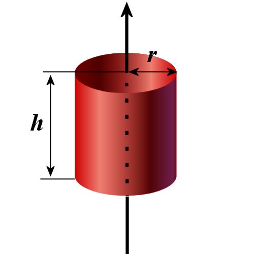
The cylindrical wall is defined using this option. The cylinder is allowed to lie along the X or Y or Z axis with the center of the cylinder on the line across the center of simulation box (the origin; (0,0,0)). In case of an infinitely long cylinder, users should prepare the cylinder potential file, which contains the following lines for all types of atom;
| {ATOM TYPE} {Rmin} {Rmax} {Filename of tabulated potential function for the ATOM TYPE} |
Rmin is the minimum radial distance of the table function from the axial center of cylinder, while Rmax is a cut-off distance.
It is also needed to give a number of data points in the file of tabulated potential.
| DIRECTION= | the direction along the cylinder axis [x, y, z] | - | - |
| FILE= | the name of the cylinder potential file | - | default: cylinder.prm |
| GRIDPOINTS= | the number of data points in the tabulated potential file | integer | 2000 |
When a cylindrical object with a finite length is used, several changes are needed. First of all, user need to declare that the cylinder is a finite length with a flag;
| FINITE_HEIGHT= | If the cylinder has a finite length, "Y", i.e., yes, otherwise "N", i.e., no. [Y/N] | - | default: N |
For a finite length cylinder, the cylinder potential file should contain the following lines for all types of atom;
| {ATOM TYPE} {Rmax} {Zmax} {Filename of tabulated potential function for the ATOM TYPE} |
Rmax is a cutoff in the radial distance and Zmax is a cutoff in the axial distance. The tabulated potential should be given to have a uniform grid in r2 in the radial direction, though r in the axial direction.
For a finite cylinder, the number of data points should be given separately for the radial and axial directions.
| NGRID_R= | the number of data points in the radial direction in the tabulated potential file | integer | 2000 |
| NGRID_H= | the number of data points in the radial direction in the tabulated potential file | integer | 2000 |
7 coloums are needed in the tabulated potential file for each atom type.
Those are;
R (radial distance), Z (axial distance from the center of cylinder), U (potential energy), dU/drxy (- force along the radial direction), dU/dz (- force along the axial direction),
dU/dr (derivative of U by the radius), dU/dh (derivative of U by the axial
length).
This 2-dimensional data should be prepared in such a way that R is changing
first with the first Z, say,
R(1), Z(1), ...
R(2), Z(1), ...
....
R(N),Z(1), ...
R(1),Z(2), ...
...
Also, R(1) = 0. and Z(1) = 0. is expected in these files.
When `continuum macroparticle model' is used, this flag is needed to specify
its radius and the number density of atoms assumed in the sphere, etc.
The
keyword for the potential mean force calculation with respect to the radius of
macroparticle is 'PMF= ON', the default value is 'PMF= OFF'.
| NUMBER= | The number of macrosphere in the system | integer | default: 1 |
| MULTIRAD= | The number of different particle radius | integer | default: 1 |
| RADIUS= | Radii of the macroparticle [Å] | real | - |
| NDENSITY= | Number density of atom assumed inside the macroparticle [Å-3] | real | default: 0.113 |
| FILE= | Parameter filename | - | default: cgsphere.prm |
| EPSILON= | The parameter ε for SPCE oxygen and carbon interaction (only for OPLS force field) [kcal/mol] | real | - |
| MACROMACRO= | The atomic LJ parameters ε[kcal/mol] and sigma [Å] for the interaction between atoms assumed to be embedded in the marcoparticle. | real | default: eps=35.23K sigma=3.55 |
The macroparticle should have the same molecular and residue name, "CGSP", and atomname should be the radii type number, which is defined in "RADIUS=" line. If you have three different radii; "MULTIRAD= 3", you needs three radii in "RADIUS" line. These three should correspond to the radii of types, 1, 2, and 3. If the colloid particle has the atomname "1", it is considered to have the size of type 1. Atomname should be defined in initial.crd file. In the parameter file (defined by the flag "FILE="), users should give "atom type name" and the tabulated potential filename for the atom type in each line. In case that the atom type is "W" (for water particle), give epsilon in Kelvin for the interaction between the macrosphere and the water particle. The tabulated potential files should have 1000 lines, assuming in each line "distance", "potential energy", "the derivative of the potential with distance", and "the derivative of the potential with sphere radius" are given.
To confine a selected molecule in a limited region between two flat walls, this keyword is useful. The wall potential is a power of the distance from the boundary, k (x-xbound)n. Between two walls, no external force is exerted on the selected molecule.
| k= | Force constant of the wall potential [kcal/mol] | real | default: 100. |
| ORDER= | The power of the wall potential function, n | integer | default: 2 |
| NSAMPLE= | Time-step interval for the output of the coordinate | real | default: 1 |
| AXIS= | The normal axis of the constraint walls [X/Y/Z] | - | - |
| REGION= | The lower and upper boundary of the non-external force region, xmin-xmax [xmin, xmax] in Å | real | - |
| ATOMS= | The selected atom numbers from i to j, namely, the selected molecule consist of the atoms numbered i to j. [i , j] | integer | - |
For the "REGION=" option, you can choose, e.g., "REGION= 18. edge", where xmax="edge" is selected. In this case, the selected molecule should be free from the external force as long as in |x|<18Å. This option is useful when you want to keep the molecule the outside of a specific region in the NPT ensemble, where the cell length is changing during the MD calculation.
The distance-dependent, electric constant is chosen by the flag. This flag is valid only for the isolated system. The electric constant, εr=4r, is used to calculate the electrostatic interaction.
When this keyword is given, an external force is applied
to the selected atoms in the amino residue. The applied potential function has
the form either
Uext(z) = E0 /
(1+(z/n)k),
or
Uext(z) = E0 /
(σ(2π)1/2) exp (-(z-μ)2/(2σ2)),
where z
denotes the membrane normal taking z=0 at the membrane center. All parameters
E0, n, k,σ, and μ are given in the parameter file defined by the
following flag.
| FILE= | parameter file | - | default: ./param/par_externalmem.prm |
By using this flag, the force exerted on selected components are stored in the files named as (Job name).FRC0001, (Job name).FRC0002, and so on. The trajectories of the selected components are also stored in the files such as (Job name).CRD0001, (Job name).CRD0002, and so on. As a default, 10,000-steps trajectories are stored in a single file. Note that, when canonical MD is performed with the SHAKE/RATTLE procedure, the constraint force cannot be taken into account in the stored intramolecular force in the current version.
| COMPONENT= | The component number of molecules to be sampled | integer | default 1 |
| FREQ= | Interval of MD step for this sampling | integer | default: - |
| DATA= | The step number of the trajectories to be stored in a file | integer | defalut: 10,000 |
To estimate the chemical potential of a molecule, thermodynamic integration scheme is used. This flag is used for such a free energy calculation. During this molecular dynamics simulation, a molecule ( assumed to be a rigid-body ) is gradually created or annihilated in the system. λ is the variable for the integration.
U(rN+1,λ) = U(rN) + λUN+1
ΔF=∫01 <UN+1>
where UN+1 is the interaction energy of the inserted molecule with the rest of the system. For details of the algorithm, user should refer to the theory section and the references therein.
| ACTION= | [CREATION, ANNIHILATION] The former flag is used to create a molecule in the system, while the latter is used to annihilate a molecule. | character | default: CREATION |
| INTERACTION= | [COULOMB, LJ, ALL] For coulomb term, the partial charge is just scaled by λ, while LJ function is modified as a scaling potential function of λ and δ. δ is the shift parameter. | character | default: ALL |
| DELTA= | The shift parameter, δ[Å2], for scaling of LJ interaction. The accuracy of the calculated free energy is sensitive to this parameter. Users should read the "Theory" section and the references therein to optimize this parameter. | real | default: 0.2 |
| COMPONENT= | The component number of the molecule to be inserted | integer | default: the last one |
| MOLNUMB= | The molecular number of the molecule to be inserted | integer | default: the last one |
| FREQ= | Interval of MD step for this sampling | integer | default: - |
| NUMSTEP= | The number of intermediate steps for the integration variable λ from 0 to 1 | integer | default: - |
| STEP= | " Step number", "λ", and "MD steps for
equilibration and for sampling" are requested with this flag. (This line should be iterated by the number of NUMSTEP) |
integer real integer integer |
default: - |
*Note: When the "COULOMB" is selected as the annihilation or creation interaction for the TI calculations, the LJ interaction of the scaled particle i is assumed to be ON (already created!). On the other hand, the "LJ" is selected, the Coulombic interaction of the scaled particle i is assumed to be OFF (annihilated: qi=0).
| >> TICR ACTION= CREATION INTERACTION= LJ DELTA= 0.2 COMPONENT= 2 MOLNUMB= 1 FREQ= 1 NUMSTEP= 10 STEP= 1 0.1 10000 100000 STEP= 2 0.2 10000 100000 STEP= 3 0.3 10000 100000 STEP= 4 0.4 10000 100000 STEP= 5 0.5 10000 100000 STEP= 6 0.6 10000 100000 STEP= 7 0.7 10000 100000 STEP= 8 0.8 10000 100000 STEP= 9 0.9 10000 100000 STEP= 10 1.0 10000 100000 << |
The size of the system box changes at a constant rate, when this option is selected. This flag may be used during equilibration MD runs. This may be useful to make a initial configuration for polymer systems, because it is not easy to make a dense polymer system without any bad contacts of atoms. In this case, after making a polymer system at a lower density, MD calculations with this flag may be used to obtain a target polymer density.
| RATE_X= | The change rate of the cell length in the x-axis [Å/ps] | real | default: 0. |
| RATE_Y= | The change rate of the cell length in the y-axis [Å/ps] | real | default: 0. |
| RATE_Z= | The change rate of the cell length in the z-axis [Å/ps] | real | default: 0. |
The minus values for these rates mean that the cell length will decrease in the direction. Note that, whenever this option is selected, the MD simulation will be carried out in canonical ensemble automatically with the conventional velocity scaling method. Again, this option may be used for an EQUILIBRATION run.
This keyword is used to apply a constraint to a group of particles to be a cluster. The definition of cluster is that any particles in the cluster are connected each other. The distance threshhold for the connection should be given. (RSH) The constraint potential is given as a cubic function and the prefactor is 20 kcal/mol.
| NUMATOM= | The number of particles in the cluster | integer | - |
| k= | Force constant [kcal/mol/A2] | real | default: 20 |
| RSH= | Threshold for the distance of connection | real | - |
| MEMBER= | The atomic numbers for all particles in the cluster (should not exceed 80 characters in a line) | integer | - |
| FE= | Free energy (PMF) calculation between the cluster and a particle[ON/OFF] | - | default: OFF |
In case of the colloidal particles, a suggested value for RSH is 2.3+2*(Radius of colloid).
When using free energy option, the following keywords are also needed.
| k_FE= | Harmonic spring constant for constraint between cluster and the particle for free energy calculation [kcal/mol/A2] | real | - |
| PAIR= | The particle (atom) number of the partner particle | integer | - |
| NSAMPLE= | Time-step interval for sampling of the constraint force | integer | default 10 |
| INITIAL= | λ(0), initial position or distance [Å] | real | - |
| RATE= | Shifting rate of the reference point or distance, V [Å/ns] | real | default - |
With RATE=0, an ordinal constraint MD will be proceeded. Non-zero rate produce a steered MD trajectory. Note that a suggested value for k_FE is different depending on the free energy method used; k_FE = 10 for steered MD, k_FE >= 100 for constraint MD.
| >>
CLUSTER NUMATOM= 10 MEMBER= 1 2 3 4 5 6 MEMBER= 7 8 9 10 RSH= 12.3 << |
This keyword is used to fix a molecule (atom) on a plane (single molecule constraint; SNGL) or to fix the distance of a pair of molecules (atoms) (pair constraint: PAIR). For a molecule, the constriant is applied to the center of mass. Note that these two different constraints cannot be used at the same time.
PAIR ((atom number) - (atom number)) ((atom number)-(atom number)) distance (real) [Å]
SNGL ((atom number) - (atom number)) direction [X/Y/Z] position (real) [Å]
Three more constraints are available. These are useful to keep atoms out of / within the defined region with clyndrical or cone shape.
CYLINDER (axis; X or Y or Z) radius (real) [Å] (atom types)
INNERCYL (axis; X or Y or Z) radius (real) [Å] (atom types)
CONE (axis; X or Y or Z) opening angle θ (real) [degree] (atom types)
Note that CYLINDER and CONE is the constraint for selected atoms to repel
from the cylindrical or cone object, i.e., the force is outward, though
INNERCYL is the constraint to keep the atoms within the CYLINDER, i.e.,
force is inward.
To calculate the constraint force, the option "NSAMPLE="
is needed. With this flag, an output file named "(JOB_NAME)F_SNGL.dat" or
"(JOB_NAME)F_PAIR.dat" will be generated.
| NSAMPLE= | Time-step interval for sampling of the constraint force | integer | - |
| k= | Harmonic spring constant [kcal/mol] | real | default: ∞ |
Note: The default value for k = ∞ means that the conventional SHAKE-like constraint method is used. Once k value given, the constraint is applied by mean of harmonic spring force. In this case, you should make sure that k is large enough for the solute to get the target position. When cylinder or cone is selected, k is set at 100.
This option is useful for a free energy calculation via thermodynamic integration scheme.
When "CONE" is selected, the overall particles will move toward
the cone tip to escape from this external force. To prevent this problem,
the center of mass (COM) of the selected particles is bind to the origin
by a harmonic constraint with k=100 kcal/mol.
When we consider the deformation of liposome using CONE potential, as opening
angle is growing, the liposome cannot stay spherical due to the constraint
on the COM. To make the liposome spherical, the COM of the seleted particles
should slightly move as changing the opening angle. The option "CORRECTCONE"
makes it possible to correct the COM position to be to keep the ideal spherical
shape of the liposome.
CORRECTCONE outer radius of liposome (real) [Å] thickness of the membrane (real) [Å]
User should give the reference data for the closed liposome; outer radius of the liposome and thickness of the liposomal membrane. In the actual calculation, we shift the cone instead of the COM position. Then, the COM of the selected particles will stay at the origin throughout the MD simulation.
| >>
OPTIONALCONSTRANT SNGL (2168-2175) Z -12.0 NSAMPLE= 10 << |
In this example, a molecule (atom group) composed of the atoms having the number from 2168 to 2175 is fixed on the x-y plane of z=-12.0.
| >>
OPTIONALCONSTRANT CONE Z 10. CM CT NSAMPLE= 10 k= 1000. CORRECTCONE 78. 30. << |
In this example, atoms whose type is CM and CT is repelled from the cone with the open angle of 20 (10 times 2) degree.
This is the keyword to use a free energy calculation technique with a steered MD using Jarzynski's equality. We can apply a constraint on a molecule (SNGL) or a pair of molecules (PAIR) with this option. A molecule or a group of atoms is selected appropriately with a option,
SNGL= ((atom number) - (atom number))
PAIR= ((atom number) - (atom number)) ((atom number)-(atom number))
Three more options are available. These are useful to force atoms to move out from or move into the defined region with clyndrical or cone shape.
CYLINDER (axis; X or Y or Z) (atom types)
INNERCYL (axis; X or Y or Z) (atom types)
CONE (axis; X or Y or Z) (atom types)
In case of CYLINDER and CONE, the force is applied for atoms outward of the objects, though in case of INNERCYL, the force is inward to keep atoms within the cylinderical geometry.
The atom types are needed to select a group of atoms interact with cylindrical or cone object. User can select "all" for (atom types) when a cavity with the shape is to be made. Note that, for CYLINDER and CONE, the selected atoms are pushed away from the object by a harmonic spring but are never attracted. This is different from SNGL and PAIR options.
In a steered MD, the guiding potential h(r,λ) = 0.5 k (ξ(r) - λ)2 (Note: for cylinder or cone option, we use cubic function instead; h(r,λ) = (1/3) k (ξ(r) - λ)3 ) is used, and the Hamiltonian of the system is
Hλ(r,p) = H(r,p) + h(r,λ)
λ is the target position or distance and is changing with time at the rate of V.
λ(t) = λ(0) + V t
During a steered MD, the work due to the external steering force, W, is measured;
| k= | Spring constant of the harmonic constraint, k [kcal/mol] | real | default 10. |
| RATE= | Shifting rate of the reference point or distance or raidus of cylinder, V [Å/ns]. For an opening angle of cone, the rate should be given in [degree/ns] | real | default - |
| NSAMPLE= | Time-step interval for output of the constraint force | integer | default 10 |
| INITIAL= | λ(0), initial position or distance or radius of cylinder [Å], or opening angle of cone θ[degree]. | real | - |
| DIRECTION= | The normal vector of the surface on which a single molecule is constrained. (x,y,z) [Å]. This option is useful for SNGL. | real | - |
After MD with this keyword, you will find W values as a function of time in the file, "(JOB_NAME)_SMD_WORK.dat". W values will be given in kcal/mol. Additionally, a file, "(JOB_NAME)_SMD_CHECK.dat" will also be generated, in which target and actual position of the constraint molecule is given.
Note that the keywords "JARZYNSKI" and "OPTIONALCONSTRAINT" are not compatible with each other, user should choose one of them.
| >> JARZYNSKI SNGL (2168-2175) NSAMPLE= 10 k= 10. RATE= 3. INITIAL= 0. DIRECTION= 0. 0. 1. << |
In this example, a molecule or a atom group composed of the atoms tagged from 2168 to 2175 is constrained on the z=0 plane initially by a harmonic spring with a strength k=10kcal/mol, and the constraint plane is shifting toward +z at the rate of 3 [Å/ns] during the MD run.
| >> JARZYNSKI CYLINDER Z CM CT NSAMPLE= 10 k= 10. RATE= 3. INITIAL= 0. << |
In this case, you will generate a cylinder along z-axis, which interact with atomic types CM and CT.
This flag is used when moment of inertia of the selected molecules are
to be controlled. The order parameter d is introduced to change the shape
of the molecular assembly.
d = 1 - 2 * e3 / (e1 + e2),
where e1, e2, and e3 are eigenvalues of the tensor of inertia. e1 and e2
have the smallest difference, i.e., |e1-e2| < |ei-ej| (i/=j) . d = 0
when the molecular assembly has a complete spherical shape. -1<d<1.
A harmonic constraint is introduced to the system, namely, the energy term,
U = 0.5 * kD * (d - d0)2
is added to the Hamiltonian. d0 is the target order parameter.
| k= | Spring constant of the harmonic constraint, kD [kcal/mol] | real | default 10. |
| d0= | target order parameter d0 (from -1 to 1) | real | default - |
| TARGET= | The component number of molecules to be controled | integer | - |
(Jobname)PMF_INERT.dat is generated during MD simulation. This file contains "time", "accumulative average of potential of mean force", "order parameter d" at each time step.
The constant electric field is applied by using this flag.
| EFIELD= | Applied electric field [V/Å] | real | default 0. |
| DIRECTION= | Direction of the applied electric field; this should be given by a vector (x, y, z) | real | default - |
This is a flag useful for calculating the electric flux from an MD simulation. With this flag, an MD yield a file, (Jobname)_Eflux.dat, which contains the electric flux of the system. (assumed the system is made of monovalent cation and anion)
| CATION= | The component number of cation | integer | default - |
| ANION= | The component number of anion | integer | default - |
This is useful only for MPDynPFF; where polarizable force field was used. The parameters control the damping function for dipole-dipole interaction.
| DAMP= | Damping factor to damp induced interactions | real | default 1.748 |
| DTOL= | Tolerance for the convergence of induced dipoles | real | default 0.001 |
| NITR= | Number of iterations for the convergence of induced dipoles | integer | default 50 |
The parameters for PIMD / CMD should be specified by using this flag.
| BEAD_LENGTH= | The length of bead | integer | default: 1 |
| REF_TIME= | The division number of the step size, γ, for the
integration of the bead elements. Δtsmall = Δt / γ is used to integrate equations of motion of the bead elements. Δt is the step size for the integration of centroid variables. |
integer | default: - |
The parameter for CMD simualtion can be modified by using this flag.
| TIME_SCALE= | Prefactor to modify time scale ( 1 / γc ) | real | default: 1.0 |
The parameters used in Hybrid MC calculations are described by this flag.
| MDSTEP= | MD steps to be performed in one MC cycle | integer | default: 10 |
| PARTIAL= | Partial momentum refreshment | [Y / N] | default: N |
| THETA= | Combination parameter for partial momentum refreshment θ [degree]* | real | default: 90.0 |
* This flag is valid only if 'PARTIAL=Y'.
| >>
HMC_PARAM MDSTEP= 20 PARTIAL= Y THETA= 45 << |
This flag is valid only when the "STATUS" is "INITIAL", used to set the step number for the equilibration term. Default value is 1000.
| STEP= | The number of step | integer | default: 1000 |
| >> EQUIL_STEP STEP= 10000 << |
This flag is used to specify the integration method of the DPD equations of motion and the dissipative parameter, γ.
| METHOD= | [VVerlet, VVerletSC, Lowe, Peters] | - | - |
| GAMMA= | γ | real | default: 4.5 |
| GAMMA_FILE= | The name of file which contain the list of γ for each pair | - | - |
| LAMBDA= | λ | real | default: 0.65 |
| ITERATION= | iteration number | real | default: 10 |
NOTE: Only in case of "VVerlet", the parameter, λ, is valid. In the case of self-consistent integrations, "VVerletSC" and "PetersSC", the number of iterative loop can be changed by "ITERATION=". For the Lowe algorithm, γ, is the parameter to determine the thermalizing collision frequency. The flag "GAMMA_FILE=" is valid only for Peters algorithm, and the file should contain the list of γ values for each pair of species in the same format as the force field data file.
| >>
INTEGRATION_DPD METHOD= VVerletSC GAMMA= 4.5 ITERATION= 5 << |
The flag is used to define the number density of the system.
| DENS= | Number density | real | default 3.0 |
| >> NDENSITY DENS= 5.0 << |
One can apply the shear field to the system with this flag. The shear field is applied at the specified shear rate by Lees-Edwards boundary condition. The default value is 0.
| >>
SHEAR_RATE 1.0 << |
This flag provides a set of trajectory files to be
analyzed.
The number of trajectory files (integer)
Header (JOBNAME) of the
trajectory file
The number of configurations, monitoring frequency
Note:
The last two lines are repeated to the number of files
| >> ANALYZ_FILE 6 ! number of files /work3/shinoda/DPPC/MD01100ps ! ## file name & step number & interval 2000 1 /work3/shinoda/DPPC/MD01410ps 6200 1 /work3/shinoda/DPPC/MD01854ps 8880 1 /work3/shinoda/DPPC/MD01878ps 480 1 /work3/shinoda/DPPC/MD02000ps 2440 1 /work3/shinoda/DPPC/MD02500ps 10000 1 << |
| METHOD= | The keyword of the analysis |
Some analyses request the additional options. The keyword and its options are listed below.
| Keyword |
PDB |
| Analysis | The configuration data are stored in the PDB format. |
| Option | STEP= The number of step integer |
| Output | snap****.pdb : **** is the step number |
| Keyword |
PDBsp |
| Analysis | The configuration of the specified components and regions in the system are stored in the PDB format. |
| Option | STEP=
Total
step number
integer NUMCOMP= The number of components selected integer SELECTED= Component number of the selected molecule integer REGION= [Y,N] default N X= region; Xmin,Xmax real default -10, 10 Y= region; Ymin,Ymax real default -10, 10 Z= region; Zmin,Zmax real default -10, 10 |
| Output | snap****.pdb : **** is the step number |
Example) The PDB file printed by the following scripts contains the configuration of the molecules, whose component numbers are 1, 3,and 5, locating in the cubic region [-20,20].
| >> ANALYZ_NAME METHOD= PDBsp STEP= 1000 NUMCOMP= 3 SELECTED= 1 3 5 REGION= Y X= -20.0 20.0 Y= -20.0 20.0 Z= -20.0 20.0 << |
| Keyword |
PDBex |
| Analysis | The molecular configuration in a specified region in the system are stored in a PDB file. |
| Option | STEP= Total step number
integer X= region; Xmin,Xmax real default - Y= region; Ymin,Ymax real default - Z= region; Zmin,Zmax real default - |
| Output | snap****.pdb : **** is the step number |
| Keyword |
PDBminR |
| Analysis | The configuration of the protein that overall translation and rotation are removed is stored as a new file in the PDB format |
| Option | STEP= Total number
of steps
integer PROTEIN= The component number of protein integer |
| Output | snap****.pdb : **** is the step number |
| Keyword |
XYZsp |
| Analysis | Convert the trajectories into a XMol file. The configuration of the components and the region specified is stored in the file, ./Analy/XMolselected.xyz, with the XMOL format. |
| Option | STEP=
Total number of steps to be stored
integer NUMCOMP= The number of components selected integer SELECTED= Component number of the selected molecule integer REGION= [Y,N] default N X= region; Xmin,Xmax real default -10, 10 Y= region; Ymin,Ymax real default -10, 10 Z= region; Zmin,Zmax real default -10, 10 |
| Output | Analy/XMolselected.xyz |
| Keyword |
CRD |
| Analysis | The configuration is stored in a new file in the CRD format. |
| Option | STEP= Total number of steps to be stored integer |
| Output | snap****.crd : **** is the step number |
| Keyword |
CBPI |
| Analysis | Chemical potential calculation by particle insertion technique with cavity-based sampling. Chemical potential profile is obtained as a function of z-axis. (For CHARMM force field only) |
| Option | FILE= Filename (the
file should contain the parameter of the molecules to be inserted.)
default: ./param/PImolecule.data T= Temperature[K] real P= Pressure [MPa] real TRIAL= The number of insertion trials at each z-value. integer default: 5 TRIORI= The number of rotational trials integer default: 10 RCAV= grid size [Å] real REGION= The region to be inserted X,Y,Z[Å] real |
| Output | CavityInsert_*.data |
| Note | Form of the file,
"./param/PImolecule.data" 1. The number of molecular species to be inserted 2. molecule 1 (A) The number of atoms (B) ε, Rminh, partial charge (for each atom) (C) Intramolecular coordinates X,Y,Z (for each atom) A blank line is needed between any two different molecular descriptions. *parallel calculation is possible |
Example:
| >>
ANALYZ_NAME METHOD= CBPI T= 323.0 P= 0.1 RCAV= 2.9 REGION= 60.0 60.0 60.0 << |
| Keyword |
Cavity |
| Analysis | (Lipid Bilayers) Analysis of the cavity distribution in the system based on the uniform cubic grid. |
| Option | LIPID=
The component number of lipid
integer RCAV= grid size [Å] real REGION= region X, Y, Z[Å] real |
| Output | distCav****.dat Cavity.dat |
| Keyword |
CorrRotW |
| Analysis | Rotational relaxation time of the TIP3P
water dipole axis. Rotational correlation function is calculated by this analysis. |
| Option | DTIME= time interval of the stored trajectory Δt[ps] real |
| Output | CorrRotationW.dat : Rotatinal correlation function #TIME[ps], P1, P2 |
| Keyword |
DiffW_Z |
| Analysis | Mean square displacements (for water molecules located at z=z, t=0) |
| Option | WATER= The component
number of water integer TOTAL= Total number of steps integer BLOCK= The number of steps per block data integer LENGTH= The length of data block for calculation of time correlation integer INTERV= Interval between data blocks integer DELTAZ= slab thickness ΔZ [Å] real DTIME= time interval of the stored trajectory Δt[ps] real MAXZ= maximum slab number to be analyzed integer MINZ= minimum slab number to be analyzed integer |
| Output | MSD_W_Z=**.dat : ##TIME[ps], MSD[Å2] |
| Keyword |
DiffMSD |
| Analysis | Mean square displacement |
| Option | NUMATM=
The number of atoms to be analyzed
integer TOTAL= Total number of steps integer BLOCK= The number of steps per block data integer LENGTH= The length of data block for calculation of time correlation integer INTERV= Interval between data blocks integer DTIME= time interval of the stored trajectory Δt [ps] real DIMENSION= dimension(Not being 3, directions should be declared) ATOM= [Atom name, residue name] (this line should be described for each atom) |
| Output | DMSD_(atomname)_(resiname).dat : ##TIME[ps], MSD[Å2] |
| Note | Usage of "DIMENSION=" DIMENSION= 3 ! ordinal MSD DIMENSION= 2 X Y ! 2 dimensional MSD in the XY plane DIMENSION= 1 Z ! 1 dimensional MSD along the z axis |
| Keyword |
DiffMSDcom |
| Analysis | Mean square displacement of molecular centers of mass |
| Option | NUMMOL= The
number of molecules to be analyzed integer
TOTAL= Total number of steps integer BLOCK= The number of steps per block data integer LENGTH= The length of data block for calculation of time correlation integer INTERV= Interval between data blocks integer DTIME= time interval of the stored trajectory Δt [ps] real DIMENSION= dimension(Not being 3, directions should be declared) MOL= [ molecule name ] ( this line should be described for each molecule ) |
| Output | DMSDcom_(molname).dat : ##TIME[ps], MSD[Å2] |
| Note | Usage of "DIMENSION=" DIMENSION= 3 ! ordinal MSD DIMENSION= 2 X Y ! 2 dimensional MSD in the XY plane DIMENSION= 1 Z ! 1 dimensional MSD along the z axis |
| Keyword | DMSD_SEL |
| Analysis | Mean square displacement of centers of mass of selected / or not-selected molecules. Selected molecules are determined by the coordination to a chosen molecule at t=0. |
| Option | NUMMOL= The
number of molecules to be analyzed integer
TOTAL= Total number of steps integer BLOCK= The number of steps per block data integer LENGTH= The length of data block for calculation of time correlation integer INTERV= Interval between data blocks integer DTIME= time interval of the stored trajectory Δt [ps] real DIMENSION= dimension(Not being 3, directions should be declared) RGCUT= (cutoff distance between the centers of mass of two molecules for the selection) [Default: 10(Å)] RCUT= (threshhold distance; a pair of atoms within this is identified to be "coordinated") MOL= [ molecule name ] and [ paired molecular name to be examined the coordination] ATOM_I= (atomnames of binding sites; give all names considered in molecule 1) ATOM_J= (atomnames of binding sites: give all names considered in molecule 2) ( the last three lines should be described for each molecule ) |
| Output | DMSDcom_(molname)_associated_(paired molname).dat : ##TIME[ps], MSD[Å2] DMSDcom_(molname)_NOT_associated_(paired molname).dat : ##TIME[ps], MSD[Å2] |
| Note | Usage of "DIMENSION=" DIMENSION= 3 ! ordinal MSD DIMENSION= 2 X Y ! 2 dimensional MSD in the XY plane DIMENSION= 1 Z ! 1 dimensional MSD along the z axis |
| Keyword |
DMSDCROSS |
| Analysis | Cross displacement of different molecules for distinct diffusion coefficient calculation. <(Ri(t)-Ri(0))・(Rj(t)-Rj(0))> |
| Option | NUMMOL= The
number of molecules to be analyzed integer
TOTAL= Total number of steps integer BLOCK= The number of steps per block data integer LENGTH= The length of data block for calculation of time correlation integer INTERV= Interval between data blocks integer DTIME= time interval of the stored trajectory Δt [ps] real DIMENSION= dimension(Not being 3, directions should be declared) MOL= [ molecule name ] ( this line should be described for each molecule ) |
| Output | DMSDcross_(molname)_(molname).dat : ##TIME[ps], MSD[Å2] |
| Note | Usage of "DIMENSION=" DIMENSION= 3 ! 3 dimensional correlation DIMENSION= 2 X Y ! 2 dimensional correlation in the xy plane DIMENSION= 1 Z ! 1 dimensional correlation along the z axis |
| Keyword |
DistRinT |
| Analysis | Distribution of travel distance of the selected molecule within a defined certain time. |
| Option | NUMMOL= The number of molecular components to be analyzed integer TOTAL= Total number of steps integer LENGTH= The number of interval steps for the distance measurement integer DTIME= time interval of the stored trajectory Δt [ps] real DIMENSION= dimension(Not being 3, directions should be declared) MOL= [ molecule name ] ( this line should be described for each molecule ) |
| Output | ./Analy/DistRT_(molname).dat : ##TIME[ps], [Å2] |
| Keyword |
VELAUTO |
| Analysis | Velocity autocorrelation function (VAF) is calculated for each specified component. |
| Option | NUMMOL= The number of molecular components to be
analyzed integer TOTAL= Total number of steps integer BLOCK= The number of steps per block data integer LENGTH= The length of data block for calculation of time correlation integer INTERV= Interval between data blocks integer DTIME= time interval of the stored trajectory Δt [ps] real DIMENSION= dimension(Not being 3, directions should be declared) MOL= [ molecule name ] ( this line should be described for each molecule ) |
| Output | ./Analy/Velauto_(molname).dat : ##TIME[ps], [Å2/ps2] |
| Note | Usage of "DIMENSION=" DIMENSION= 3 ! ordinal VAF DIMENSION= 2 X Y ! 2 dimensional VAF in the XY plane DIMENSION= 1 Z ! 1 dimensional VAF along the z axis |
| Keyword |
VELCROSS |
| Analysis | Velocity crosscorrelation function (VCF) is calculated for all specified components. |
| Option | NUMMOL= The number of molecular components to be
analyzed integer TOTAL= Total number of steps integer BLOCK= The number of steps per block data integer LENGTH= The length of data block for calculation of time correlation integer INTERV= Interval between data blocks integer DTIME= time interval of the stored trajectory Δt [ps] real DIMENSION= dimension(Not being 3, directions should be declared) MOL= [ molecule name ] ( this line should be described for each molecule ) |
| Output | ./Analy/Velcross_(molname).dat : ##TIME[ps], [Å2/ps2] |
| Note | Usage of "DIMENSION=" DIMENSION= 3 ! ordinal VCF DIMENSION= 2 X Y ! 2 dimensional VCF in the XY plane DIMENSION= 1 Z ! 1 dimensional VCF along the z axis |
| Keyword |
LifeTimeW |
| Analysis | Lifetime of the bound water |
| Option | WATER=
The component number of
water integer
NUMCOOR= The number of hydrated atoms integer RC= cut-off radius [Å] real TOTAL= Total number of steps integer BLOCK= The number of steps per block data integer LENGTH= The length of data block for calculation of time correlation integer INTERV= Interval between data blocks integer DTIME= time interval of the stored trajectory Δt [ps] real ATOM= [ atom number, residue number ] integer (this line should be described for each atom) |
| Output | LifeTimeW.dat : Residence time correlation function (see Shinoda et al. J. Phys. Chem. B 107, 14030 (2003).) |
| Keyword | LifeTime |
| Analysis | Lifetime of the bound pairs |
| Option | NUMPAIR= The number of pairs integer TOTAL= Total number of steps integer BLOCK= The number of steps per block data integer LENGTH= The length of data block for calculation of time correlation integer INTERV= Interval between data blocks integer DTIME= time interval of the stored trajectory Δt [ps] real PAIR= atom name(i), residue name(i), atom name(j), residue name(j), cutoff radius [Å] ( this line should be described for each pair ) NOINTRA= [ON/OFF] : this option may be used when user wants to eliminate the intramolecular contribution to the distribution function. "NOINTRA= ON" means the intramolecular distribution is excluded from the calculation. Default : ON. REBIND= [ON/OFF] : this option is used to define how to treat the rebinding pairs. When ON is chosen, the pairs rebind after separted will be taken into account. OFF means that the rebound pairs are not considered; once the pairs separted, the pairs will not be cosidered survived. Default : ON |
| Output | LifeCorr_**_**-**_**.dat : Residence time correlation function |
| Keyword |
RDF |
| Analysis | radial distribution function |
| Option | NUMPAIR= The
number of pairs
integer RC= Cut-off radius [Å] real GRID= grid size [Å] real PAIR= [atom name(i), residue name(i), atom name(j), residue name(j)] ( this line should be described for each pair ) NOINTRA= [ON/OFF] : this option may be used when user wants to eliminate the intramolecular contribution to the distribution function. "NOINTRA= ON" means the intramolecular distribution is excluded from the calculation. Default : OFF. |
| Output | GR_**_**-**_**.dat |
| Note | User can specified the atom pairs by using an abbreviation. When the initials of the atom name is used, all atoms belong to the same residue is selected. For example, for TIP3P water, in case of the abbreviation "H" is used, both "H1" and "H2" will be selected in the RDF calculation. *This analysis can be conducted by using multiple processors. |
| Keyword |
RDFG |
| Analysis | radial distribution function between molecular COM(center of mass)s |
| Option | NUMPAIR= The number of pairs
integer RC= Cut-off radius [Å] real GRID= grid size [Å] real PAIR= [residue(molecular) name(i), residue(molecular) name(j)] ( this line should be described for each pair ) |
| Output | GR_**-**.dat |
| Keyword |
RZ |
| Analysis | Probability distribution of the selected atom along the specified axis. |
| Option | AXIS=
The
axis to which the atom position projected.
[ X / Y / Z ] RANGE= Range for the analysis [ Min. Max. ] ( from Min to Max ) GRID= The slab size, Δ NUMATOM= The number of the selected atoms for the analysis ATOM= [atom name, residue name] (The line 'ATOM=' should be described for each atom) |
| Output | RZ_(AtomName)_(ResiName).dat |
| Note | By using an abridged notation for the atoms, plural atoms are selected at the same time. This is valid only when the initials of all atoms to be selected are the same and the all atoms belong to the same residue. For example, for TIP3P water, in case of the abbreviation "H" is used for the atom name, both "H1" and "H2" will be selected in the calculation. |
| Keyword |
RZG |
| Analysis | Probability distribution of the COM of the selected molecule (residue) along the specified axis. |
| Option | AXIS=
The
axis to which the atom position projected.
[ X / Y / Z ] RANGE= Range for the analysis [ Min. Max. ] ( from Min to Max ) GRID= The slab size, Δ NUMMOL= The number of the selected atoms for the analysis MOL= [residue name] (The line 'MOL=' should be described for each atom) |
| Output | RZ_(AtomName)_(ResiName).dat |
| Note | By using an abridged notation for the atoms, plural atoms are selected at the same time. This is valid only when the initials of all atoms to be selected are the same and the all atoms belong to the same residue. For example, for TIP3P water, in case of the abbreviation "H" is used for the atom name, both "H1" and "H2" will be selected in the calculation. |
| Keyword |
RD |
| Analysis | Radial distribution of the selected atom from the center of the simulation box |
| Option | RANGE=
Range for the
analysis [ Min. Max. ] ( from Min to Max ) GRID= The slab size, Δ NUMATOM= The number of the selected atoms for the analysis ATOM= [atom name, residue name] (The line 'ATOM=' should be described for each atom) CORRCOM= The component number whose center of mass is set to the origin during the analysis. This is an optional and works when it is selected. |
| Output | RD_(AtomName)_(ResiName).dat |
| Note | By using an abridged notation for the atoms, plural atoms are selected at the same time. This is valid only when the initials of all atoms to be selected are the same and the all atoms belong to the same residue. For example, for TIP3P water, in case of the abbreviation "H" is used for the atom name, both "H1" and "H2" will be selected in the calculation. |
| Keyword |
RDdisk |
| Analysis | 2-dimensional radial distribution of the selected atom from the center of the simulation box |
| Option | RANGE=
Range for the
analysis [ Min. Max. ] ( from Min to Max ) GRID= The slab size, Δ NUMATOM= The number of the selected atoms for the analysis AXIS= The normal axis [X/Y/Z] ATOM= [atom name, residue name] (The line 'ATOM=' should be described for each atom) |
| Output | RDdisk_(AtomName)_(ResiName).dat |
| Note | By using an abridged notation for the atoms, plural atoms are selected at the same time. This is valid only when the initials of all atoms to be selected are the same and the all atoms belong to the same residue. For example, for TIP3P water, in case of the abbreviation "H" is used for the atom name, both "H1" and "H2" will be selected in the calculation. |
| Keyword |
RDdiskCOM |
| Analysis | 2-dimensional radial distribution of the COM of the selected molecules from the center of the simulation box |
| Option | RANGE=
Range for the
analysis [ Min. Max. ] ( from Min to Max ) GRID= The slab size, Δ NUMMOL= The number of the selected molecules for the analysis AXIS= The normal axis [X/Y/Z] MOL= [residue (molecular) name] (The line 'MOL=' should be described for each atom) |
| Output | RDdiskCOM_(ResiName).dat |
| Note | By using an abridged notation for the atoms, plural atoms are selected at the same time. This is valid only when the initials of all atoms to be selected are the same and the all atoms belong to the same residue. For example, for TIP3P water, in case of the abbreviation "H" is used for the atom name, both "H1" and "H2" will be selected in the calculation. |
| Keyword |
RZCyl |
| Analysis | The probability distribution of the selected atoms along the Z-axis is calculated. This analysis is carried out for atoms inside and outside the cylinder whose center is located at the center of mass of the reference molecule. This analysis is useful for ion channel systems. |
| Option | NUMATOM= The number of
selected atoms integer ATOM= [atom name, residue name] (this line should be described for each atom) REFMOL= The component number of the molecule that defines the cylinder integer RADIUS= The radius of the cylinder [Å] real |
| Output | RZint_(AtomName)_(ResiName).dat RZout_(AtomName)_(ResiName).dat |
| Keyword |
RZRes |
| Analysis | Probability density of the centers of mass of the residues along the z-axis is calculated. |
| Option | NUMRES= The
number of residue to be calculated integer
RESIDUE= Residue number integer (this line should be described for each residue) |
| Output | RZ(Residue Number).dat |
| Keyword |
RZResG |
| Analysis | Probability density of the residual centers of mass along the z-axis is calculated. The origin of the z-axis is chosen at the protein center of mass. |
| Option | NUMRES=
The number of residue to be
calculated integer
RESIDUE= Residue number integer (this line should be described for each residue) REFMOL= Component number of the protein, which defines the origin of the z-axis integer |
| Output | RZG(Residue Number).dat |
| Keyword |
ResidTrj |
| Analysis | Make a trajectory file for selected residues |
| Option | NUMRES= The number of residue to be
calculated integer RESIDUE= Residue number integer (this line should be described for each residue) |
| Output | ResTraj***.dat |
| Keyword |
WatOrient |
| Analysis | Density and averaged orientational profiles of water molecules along the z-axis. |
| Option | - |
| Output | DensWater.dat OriWater.dat |
| Keyword |
MSD_P, MSD_Pr, MSD_Pm |
| Analysis | Time evolution of averaged MSD of Cα of the protein. By using options "SP=", MSD of the selected residue can be evaluated. (MSD_PrD: rotational correction, MSD_PmD: minimized MSD by rotational correction) |
| Option | PROTEIN= The component
number of protein molecule
integer SP= The first residue number, the last residue number integer (repeat this line if necessary) |
| Output | MSD_protein.dat MSD_proteinR.dat MSD_Minim.dat |
| Keyword |
MSD_PD, MSD_PrD, MSD_PmD |
| Analysis | Root mean deviation of Cα atoms of proteins. Each residue is separately evaluated. The option "SP=" is used to specify the transmenbrane region. (MSD_PrD: rotational correction, MSD_PmD: minimized MSD by rotational correction) |
| Option | PROTEIN= The component
number of protein molecule
integer
SP= The first residue number, the last residue number integer (repeat this line if necessary) |
| Output | MSD_proteinRD.dat MSD_Minim_detail.dat |
| Keyword |
MSD_PmD_MS |
| Analysis | Time evolution of MSD of the main chain (N,C,Cα) and side chains of the protein. The calculated MSD is minimized by translational and rotational operations. Trajectory of the protein centers of mass and the averaged conformation of the protein are also obtained |
| Option | PROTEIN= The component number of protein molecule integer |
| Output | ProteinAvConf.dat TrajProtCOM.dat RMSD_Min_MainChain.dat RMSD_Min_SideChain.dat |
| Keyword |
RofG_Prot |
| Analysis | Radius of gyration of the protein molecule |
| Option | PROTEIN= The component number of protein molecule integer |
| Output | RofG_Protein.dat |
| Keyword |
VoronoiL, VoronoiC |
| Analysis | 2-dimensional Voronoi analysis for the lipid centers of mass (VoronoiL) and the hydrophobic chain centers of mass (VoronoiC) in the bilayer plane. Voronoi area, its distribution, and the number of side of the Voronoi polygon. |
| Option | LIPID= The component number of lipid integer |
| Output | Vor_Area.dat Vor_Side.dat Dis_Side.dat PolygonLupp.dat PolygonLlow.dat Rg.dat Rupp.dat Rlow.dat |
| Keyword |
TraceG |
| Analysis | Trajectory of the centers of mass of the selected molecule |
| Option | MOLNUM=
Component number of the selected molecule
integer FREQ= Step interval for output integer |
| Output | TraceG.dat |
| Keyword | TrajCOM |
| Analysis | Trajectory of the centers of mass of the selected molecule |
| Option | SELECTC= [Y/N] for each components FREQ= Step interval for output integer |
| Output | TrajCOM#.dat : # is the component number |
| Comment | example) SELECTC= Y Y N means that you have three components in the system and selected the first two components for this analysis. This yields the trajectories of the centers of mass of molecules of the first two componts. |
| Keyword |
LS_anim |
| Analysis | PDB trajectory file of the selected, one lipid molecule |
| Option | NUMLIPID= The molecule number of the selected lipid integer |
| Output | snap**.pdb
Rg** |
| Keyword |
ElecZ |
| Analysis | Electrostatic potential, polarization, and charge density profile along the bilayer normal. |
| Option | - |
| Output | ElecPhiS.dat (electrostatic
potential) ElecPotS.dat (polarization) ElecRhoS.dat (charge density) |
| Keyword |
Edens |
| Analysis | Electron density profile along the bilayer normal. |
| Option | AXIS=
The
axis to which the atom position projected.
[ X / Y / Z ] RANGE= Range for the analysis [ Min. Max. ] ( from Min to Max ) GRID= The slab size, Δ |
| Output | ElectronDensityZ.dat |
| Keyword |
SCD |
| Analysis | Order parameter profile of the acyl chains of LIPID (DPPC/DPhPC/DMPC/PtPC/TEPC/TBPC/POPC/POPS/DOPC/SDS/DTDA/SPM2/SM18/LSM/PGPM) |
| Option | - |
| Output | SCD.dat |
| Keyword |
SmolB |
| Analysis | Segmental order parameter profile of the acyl chains of LIPID (DPPC/DPhPC) |
| Option | - |
| Output | SmolB.dat |
| Keyword |
FracGauche |
| Analysis | Ratio of the gauche defect observed along the hydrophobic main chain of the (DPPC/DPhPC/DMPC) lipid molecules |
| Option | - |
| Output | Ave_GaucheFrac.dat GaucheFrac.dat |
| Keyword |
OriChain |
| Analysis | Distribution and time correlation of orientation of alkyl chain of the lipid molecules(DPPC,DPhPC) |
| Option | DTIME= time interval of the stored trajectory Δt[ps] real |
| Output | DisChain_*_*.dat CorrChain_*_*.dat |
| Keyword |
LenChain |
| Analysis | distribution and time correlation of length of alkyl chain of the lipid molecules(DPPC,DPhPC) |
| Option | DTIME= time interval of the stored trajectory Δt[ps] real |
| Output | DisChainLength_*_*.dat CorrChainLength_*_*.dat |
| Note | Analysis of auto-correlation function still has some bugs. |
| Keyword |
CoTGLipidC |
| Analysis | Time correlation function of trans-gauche isomerizations of dihedrals in the acyl chains of LIPID |
| Option | TOTAL= Total
number of steps integer
BLOCK= The number of steps per block data integer LENGTH= The length of data block for calculation of time correlation integer INTERV= Interval between data blocks integer DTIME= time interval of the stored trajectory Δt[ps] real |
| Output | Cotg_Gamm_Dih_**.dat Cotg_Beta_Dih_**.dat GaucheCheck.dat |
| Note | only for DPPC, DMPC, PhPC(DPhPC) |
| Keyword |
GR_LipidGG |
| Analysis | 2-dimensional radial distribution function between lipid centers of mass in the bilayer plane. |
| Option | LIPID= The component number of lipid
integer RC= cut-off radius [A] |
| Output | GR_LipidGG.dat |
| Keyword |
WatOrientG |
| Analysis | Density and averaged orientational profiles of water molecules (center of mass) along the z-axis. |
| Option | - |
| Output | DensWater_inCylG.dat
DensWater_outCylG.dat OriWater_inCylG.dat OriWater_outCylG.dat |
| Keyword |
WatOriCyl |
| Analysis | Density and averaged orientational profiles of water molecules along the z-axis is calculated separately inside and outside of the cylinder. |
| Option | PROTEIN= The component
number of protein molecule integer
RADIUS= The radius of the cylinder [A] real |
| Output | DensWater_inCylG.dat
DensWater_outCylG.dat OriWater_inCylG.dat OriWater_outCylG.dat |
| Keyword |
WatOriCylG |
| Analysis | Density and averaged orientational profiles of water molecules along the z-axis is calculated separately inside and outside of the cylinder. |
| Option | PROTEIN= The component
number of protein molecule integer
RADIUS= The radius of the cylinder [A] real |
| Output | DensWater_inCylG.dat
DensWater_outCylG.dat OriWater_inCylG.dat OriWater_outCylG.dat |
| Keyword |
PoreWatTrj |
| Analysis | Trajectory of the water molecules that migrate in the cylinder whose center is located at the center of mass of the reference (protein) molecule. |
| Option | PROTEIN= The component
number of protein molecule integer
RADIUS= The radius of the cylinder [A] real LENGTH= The length of the cylinder [A] real |
| Output | NumWatPore.dat
WatTraj****.dat |
| Keyword |
PoreWater |
| Analysis | Probability histogram and trajectory of the water molecules that exist in the cylinder whose center is located at the center of mass of the reference (protein) molecule. |
| Option | PROTEIN= The component
number of protein molecule integer
RADIUS= The radius of the cylinder [A] real LENGTH= The length of the cylinder [A] real |
| Output | GridDensityWater.dat
WatTraj****.dat |
| Keyword |
CGdata |
| Analysis | Sampling data for coarse-graininig of the lipid bilayer system. |
| Option | RC=
Rutoff radius [A]
real
default: the value in the flag
of PBC TEXT= Temperature [K] real default: 303K |
| Output | CGconfig.dat (centers of mass of coarse
grained sites / binary) Bond*--*.dat (probability distribution of bond length and the effective potential) Angle*--*--*.dat (probability distribution of bending angle and the effective potential) GR*--*.dat (radial distribution function between CG sites.) |
| Keyword |
CGAlkane |
| Analysis | Sampling data for coarse-graininig of the alkane system. |
| Option | RC= Rutoff radius [A] real default: the value in the flag of PBC |
| Output | Bond*--*.dat Angle*--*--*.dat GR*--*.dat |
| Keyword | ID_MICELLE |
| Analysis | Cluster analysis for micellar solution |
| Option | DISTANCE=
Threshold of bonded distance [A]
real LIPID= The component number of lipid or surfactant |
| Output |
| Keyword | ZANGLEmem |
| Analysis | Orientation of the selected vector connecting two atoms (I and J) within the same molecule with respect to the outerward membrane normal vector |
| Option | PAIR [Molname] [Atom I] [Atom J] |
| Output | distcos_[Atom I]--[Atom J]_[Atom K].dat (in cos θ)
distcos2_[Atom I]--[Atom J]_[Atom K].dat (in cos2 θ) distangle_[Atom I]--[Atom J]_[Atom K].dat (in θ[degree]) |
| Keyword | RELANGLE |
| Analysis | Angular distribution of two selected vectors connecting two atoms (I and J) within the same molecule |
| Option | PAIR [Molname] [Atom I] [Atom J] [Atom K] [Atom L] Example) 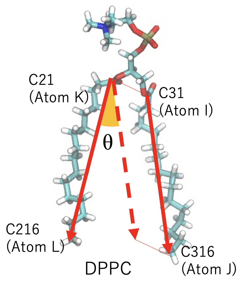 PAIR DPPC C31 C316 C21 C216 Note: you can have many these lines as you want. |
| Output | distcos_[Atom I]--[Atom J]_[Atom K]--[Atom L]_[Molname].dat (in
cos θ) distcos2_[Atom I]--[Atom J]_[Atom K]--[Atom L]_[Molname].dat (in cos2 θ) distangle_[Atom I]--[Atom J]_[Atom K]--[Atom L]_[Molname].dat (in θ[degree]) |
| Keyword |
dPP |
| Analysis | P-P Distance in the lipid bilayer |
| Option | - |
| Output | dPP.dat |
| Keyword |
CGW |
| Analysis | Analysis for structure and energy between water-water for AA model to generate a coarse-grained model |
| Option | RC= Rutoff radius [A] real default: the value in the flag of PBC |
| Output | ene_blob_intra.dat (intrablob energy
(nonbond) / binary) ene_blob_intra_bound.dat (maximum and minimum energy) gr_blob_mol.dat (gr of water molecules agains blob) ene_blob_mol.dat (interaction energy beween a molecule and a blob) ene_blob_blob.dat (interaction energy between blobs) gr_blob_blob.dat (gr between blobs) |
| Keyword |
CGchainW |
| Analysis | Analysis for energy between CG sites in chain molecule and blob water |
| Option | RC= Rutoff radius [A] real default: the value in the flag of PBC |
| Output | Ene_Type*--blobW.dat |
| Keyword |
DISTinMOL |
| Analysis | Analysis for probability distribution of bond lengths, angles, dihedral angles in a molecule. |
| Option | The bond, angle, dihedral pairs should
be given in each line, with the options starting from "BOND", "ANGLE",
"DIHEDRAL", respectively. BOND [Molecule name] (Atomname 1) (Atomname 2) ANGLE [Molecule name] (Atom 2) (Atom 2) (Atom 3) DIHEDRAL [Molecule name] (Atom 1) (Atom 2) (Atom 3) (Atom 4) RGRID= grid size for distance [A] real default: 0.1A DGRID= grid size for angles [degree] real default: 1 degree In addition, a data range for a distribution calculation is selected with the following options; RRANGE= minimum and maximum distances [A] real default : 2 and 8A |
| Output | disbond_(Atom1)--(Atom2)_(Molecule
name).dat disangle_(Atom1)--(Atom2)--(Atom3)_(Molecule name).dat disdihedral_(Atom1)--(Atom2)--(Atom3)--(Atom4)_(Molecule name).dat |
| Keyword |
Rot5Ring |
| Analysis | Rotational relaxation analysis for 5-membered ring (calculating P2 time correlation function) |
| Option | MOLNAME= (molecular name) ATOMS= (five atomnames making the target ring) give all names in one line DTIME= time interval of the stored trajectory Δt[ps] real 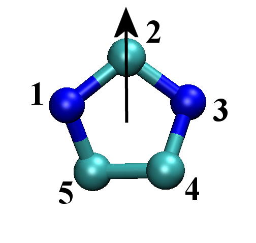 Note that P2 relaxation of the vector connecting the center of mass of the ring and the 2-nd atom is analyzed. |
| Output | Analy/Rot_Ring_(MOLNAME).dat |
| Keyword |
Rot5RingSL |
| Analysis | Rotational relaxation analysis for 5-membered ring of the selected / or not-selected molecules. Selected molecules are determined by the coordination to a chosen molecule at t=0. (calculating P2 time correlation function) |
| Option | MOLNAME= (molecular name) and [ paired
molecular name to be examined the coordination] ATOMS= (five atomnames making the target ring) give all names in one line DTIME= time interval of the stored trajectory Δt[ps] real RGCUT= (cutoff distance between the centers of mass of two molecules for the selection) [Default: 10(Å)] RCUT= (threshhold distance; a pair of atoms within this is identified to be "coordinated") ATOM_I= (atomnames of binding sites; give all names considered in molecule 1) ATOM_J= (atomnames of binding sites: give all names considered in molecule 2) TOTAL= Total number of steps integer BLOCK= The number of steps per block data integer LENGTH= The length of data block for calculation of time correlation integer INTERV= Interval between data blocks integer Note that P2 relaxation of the vector connecting the center of mass of the ring and the 2-nd atom is analyzed. |
| Output | Analy/Rot_Ring_(MOLNAME)_associated_(paired molname).dat Analy/Rot_Ring_(MOLNAME)_NOT_associated_(paired molname).dat |
| Keyword |
RotVec |
| Analysis | Rotational relaxation analysis for a vector connecting specified two atoms (calculating P1, P2 time correlation function) |
| Option | MOLNAME= (molecular name) ATOMS= (two atomnames) give all names in one line DTIME= time interval of the stored trajectory Δt[ps] real Note that the rotational relaxation of the vector connecting atom 1 to atom 2 is analyzed. |
| Output | Analy/Rot_Vec_(Atom1)-(Atom2).dat |
| Keyword |
RotVec_SEL |
| Analysis | Rotational relaxation analysis for a vector connecting specified two atoms in the selected / or not-selected molecules. Selected molecules are determined by the coordination to a chosen molecule at t=0. (calculating P1, P2 time correlation function) |
| Option | MOLNAME= (molecular name) and [ paired
molecular name to be examined the coordination] ATOMS= (two atomnames) give all names in one line TOTAL= Total number of steps integer BLOCK= The number of steps per block data integer LENGTH= The length of data block for calculation of time correlation integer INTERV= Interval between data blocks integer DTIME= time interval of the stored trajectory Δt[ps] real RGCUT= (cutoff distance between the centers of mass of two molecules for the selection) [Default: 10(Å)] RCUT= (threshhold distance; a pair of atoms within this is identified to be "coordinated") ATOM_I= (atomnames of binding sites; give all names considered in molecule 1) ATOM_J= (atomnames of binding sites: give all names considered in molecule 2) Note that the rotational relaxation of the vector connecting atom 1 to atom 2 is analyzed. |
| Output | Analy/Rot_Vec_(Atom1)-(Atom2)_(molname)_associated_(paired molname).dat Analy/Rot_Vec_(Atom1)-(Atom2)_(molname)_NOT_associated_(paired molname).dat |
| Keyword |
Rot3v |
| Analysis | Rotational relaxation analysis for a unit vector of R21 + R23 (calculating P1, P2 time correlation function) |
| Option | MOLNAME= (molecular name) ATOMS= (three atomnames) give all names in one line DTIME= time interval of the stored trajectory Δt[ps] real Note that the rotational relaxation of the unit vector of R21 + R23 is analyzed. (assuming the dipole vector of water) |
| Output | Analy/Rot_3v_(Molname).dat |
| Keyword |
Rot3v_SEL |
| Analysis | Rotational relaxation analysis for a unit vector of R21 + R23 (calculating P1, P2 time correlation function) |
| Option | MOLNAME= (molecular name) and [ paired
molecular name to be examined the coordination] ATOMS= (three atomnames) give all names in one line DTIME= time interval of the stored trajectory Δt[ps] real TOTAL= Total number of steps integer BLOCK= The number of steps per block data integer LENGTH= The length of data block for calculation of time correlation integer INTERV= Interval between data blocks integer RGCUT= (cutoff distance between the centers of mass of two molecules for the selection) [Default: 10(Å)] RCUT= (threshhold distance; a pair of atoms within this is identified to be "coordinated") ATOM_I= (atomnames of binding sites; give all names considered in molecule 1) ATOM_J= (atomnames of binding sites: give all names considered in molecule 2) Note that the rotational relaxation of the unit vector of R21 + R23 is analyzed. (assuming the dipole vector of water) |
| Output | Analy/Rot_3v_(Molname).dat |
| Keyword | INERTMOM |
| Analysis | Analyze moment of inertia of the selected species |
| Option | TARGET= (The component number of the selected molecules) |
| Output | Analy/MomentOfInertia.dat |
| Keyword | COORDIS |
| Analysis | Coordination number between two molecules (assuming these molecules have
multiple interaction sites) for pairs within a cut-off distance. The coordination
number is given as a smooth function of the distance of pairs of interacting
sites: 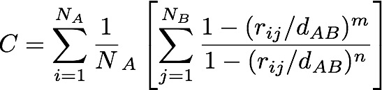 m should be smaller than n. d_AB is the scale parameter. m=6, n=12 are the default values. In this analysis, a histogram of the coordination numbers as a function of distance between the centers of mass of two molecules. |
| Option | MOLNAMES= (a pair of molecular (residue) names should be given; molecules 1 and
2) ATOM_I= (atomnames of binding sites; give all names considered in molecule 1) ATOM_J= (atomnames of binding sites: give all names considered in molecule 2) RGCUT= (cutoff distance between the centers of mass of two molecules) DR= (grid size of histogram) M= (exponent in the above equation; default: 6) N= (exponent in the above equation; default: 12) D= (the sale parameter d_AB in the above expression) |
| Output | Analy/CoorDis.dat, Analy/CoorDisAv.dat |
| Keyword | COORPAIR |
| Analysis | Coordinated pair list between molecules (assuming these molecules have multiple interaction sites) within a cut-off distance is made by this analysis. The cutoff distance for COMs (RGCUT) is used for an computational efficiency. The atom pairs existing within the distance RCUT are recognized to be coordinated. This analysis yields the "coordinated" pair list. |
| Option | MOLNAMES= (a pair of molecular (residue) names should be given; molecules 1 and
2) ATOM_I= (atomnames of binding sites; give all names considered in molecule 1) ATOM_J= (atomnames of binding sites: give all names considered in molecule 2) RGCUT= (cutoff distance between the centers of mass of two molecules) [Default: 10(Å)] RCUT= (threshhold distance; a pair of atoms within this is identified to be "coordinated") |
| Output | Analy/CoorPair.dat |
| Keyword | COORPAIRG |
| Analysis | Coordinated pair list between molecules within a cut-off distance of COMs is made by this analysis. This analysis yields the "coordinated" pair list. |
| Option | MOLNAMES= (a pair of molecular (residue) names should be given; molecules 1 and
2) RGCUT= (cutoff distance between the centers of mass of two molecules) |
| Output | Analy/CoorPairG.dat |
| Keyword | NSPHERE |
| Analysis | Analyze the number of molecules (particles) within a sphere with a given radius and the ceter at the origin. |
| Option | RADIUS= (the radius of sphere in [A]) MOLNAME= (molecular name to be analyzed) |
| Output | Analy/Nsphere.dat |
| Keyword | STRESSPROF |
| Analysis | Stress profile computation along the z-axis (useful only for CG models) |
| Option | CONTOUR= [IK/HARASHIMA] (Irvin-Kirkwood or Harashima contour) NGRID= The number of bins EWALD= [ON/OFF] (when it is ON, the parameters for Ewald can be changed in the keyword, "COULOMB") RCC= Cut-off length of coulomb interaction [default: equal to vdw cutoff length] GEOMETRY= [SPHERICAL,PLANER] (definition of the shape of the silces; default:PLANER) RBIN= The bin width of the spherical slices (for SPHERICAL bins only) CORRCOM= The component number whose center of mass is set to the origin during the analysis. This is an optional and works when it is selected. |
| Output | Analy/StressProfile.dat |
| Note | For spherical geometry, IK is the only option for the computation. |
| Keyword | ELECOND |
| Analysis | Electro-conductivity measurement based on the analysis of the velocity autocorrelation funtion. |
| Option | TOTAL= Total number of steps integer BLOCK= The number of steps per block data integer LENGTH= The length of data block for calculation of time correlation integer INTERV= Interval between data blocks integer DTIME= time interval of the stored trajectory Δt [ps] real |
| Output | Analy/Elecond.dat |
| Note |
| Keyword | HBONDS |
| Analysis | Analysis for hydrogen bonding pair (how many and how long) |
| Option | NDONER= Number of proton doners NACCEPTOR= Number of proton acceptors RC= The criterion for the distance between two heavy atoms [A] THETA= The criteron for the angle for hydrogen bonding [degree] (default 30 degree) NOINTRA= [ON/OFF] : this option may be used when user wants to exclude the hydrogen bonding within the same molecule. "NOINTRA= ON" means the intramolecular hydrogen bond is excluded from the calculation. Default : OFF. The following two options are needed for all doners and acceptors. Each one have to be described in one line, so the line should be repeated by the number of doner and acceptor types. DONER= Proton doner (a pair of atoms (together with hydrogen) and molecule names should be given) ACCEPTOR= Proton acceptor (atom and molecule names should be given) LIFETIME= [ON/OFF] : If this is ON, a calculation to estimate the life time of hydrogen bonding will be done. Only when this option is ON, the following options are needed. [De TOTAL= Total number of steps integer BLOCK= The number of steps per block data integer LENGTH= The length of data block for calculation of time correlation integer INTERV= Interval between data blocks integer DTIME= time interval of the stored trajectory Δt [ps] real REBIND= [ON/OFF] : this option is used to define how to treat the rebinding pairs. When ON is chosen, the pairs rebind after separted will be taken into account. OFF means that the rebound pairs are not considered; once the pairs separted, the pairs will not be cosidered survived. Default : ON |
| Output | Analy/Hbonds.dat, Analy/Lifetime_hbond.dat |
| Note | If the atomname is given with a single character, all atomnames starting
from the character are considered for the analysis. Example: NDONER=1 NACCEPTOR=1 DONER= OH2 H TIP3 ACCEPTOR= OH2 TIP3 In this case, both "H1" and "H2" are considered. Namely, hydrogen bonds between OH2-H1and OH2 as well as between OH2-H2 and OH2 are taken into account when searching the hydrogen bonding pairs. Namely, this is the same as; NDONER=2 NACCEPTOR=1 DONER= OH2 H1 TIP3 DONER= OH2 H2 TIP3 ACCEPTOR= OH2 TIP3 |
| Keyword | GR_LipidGG |
| Analysis | Two dimensional radial distribution function among lipid centers of mass within the same leaflet of bilayer |
| Option | NUMLIPID= Number of lipid species to be analyzed integer
NUMLAYER= The number of leaflets analyzed separately integer RC= Rut-off length of the RDF calculations [A] real GRID= Grid size of histogram [A] real LIPID= Molecular name of the lipid to be analyzed (repeat for all lipids) |
| Output | Analy/GR2_GG_(lipid name)--(lipid name).dat |
| Note | Files to define which molecules belong to which layer. The file is required
for each lipid. If you have DPPC, the filename should be "DPPC.layer".
This file contains a list of molecular numbers with a identification of
the number of layer. Example) when DPPC molecules (1-64) forms a leaflet and molecules (65-128) forms the other leaflet, "DPPC.layer" should contains the following two lines; [1] 1-64 [2] 65-128 The numbers in [ ] is the layer number, and the range of numbers in the same line give the molecular numbers of the molecules that belong to the layer. The analysis calculates the RDF averaged over all layers. |
| Keyword | SUSCEPT |
| Analysis | Susceptibility measurement using autocorrelation function of system dipolemoment. The dipole moment was decomposed into two terms; Corrective rotation of dipole with respect to COM and corrective translational mode of COM of each molecule. |
| Option | TOTAL= Total number of steps integer BLOCK= The number of steps per block data integer LENGTH= The length of data block for calculation of time correlation integer INTERV= Interval between data blocks integer DTIME= time interval of the stored trajectory Δt [ps] real |
| Output | Analy/dipMJ.dat Analy/corr_MM.dat Analy/corr_MJ.dat Analy/corr_JM.dat Analy/corr_JJ.dat |
| Note | For more details, refer to Shim and Kim, J. Phys. Chem. B, 112, 11028 (2008). |
| Keyword | DIPMROT |
| Analysis | Susceptibility measurement using autocorrelation function of system dipole moment from corrective rotation of dipole with respect to COM of each molecule. |
| Option | TOTAL= Total number of steps integer BLOCK= The number of steps per block data integer LENGTH= The length of data block for calculation of time correlation integer INTERV= Interval between data blocks integer DTIME= time interval of the stored trajectory Δt [ps] real |
| Output | Analy/dipMJ.dat Analy/corr_MM.dat Analy/corr_MJ.dat Analy/corr_JM.dat Analy/corr_JJ.dat |
| Note | For more details, refer to Shim and Kim, J. Phys. Chem. B, 112, 11028 (2008). |
| Keyword | ENERGYHIST |
| Analysis | Energy histogram analysis for chemical potential calculation using Energy Representation Method |
| Option | INSERTION= [Y/N] |
| Output | Analy/StressProfile.dat |
| Note |