Tutorial / Example
All files needed are supplied in MPDyn/case_study/ElecSol_MD/NaClsoln
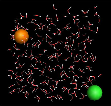
System
| TIP3P (water) |
254 molecules |
| Na+ (sodium ion) |
1 |
| Cl- (chloride ion) |
1 |
Inputs
- Preparation of the initial configuration file: At first one has to prepare
the configuration file in the PDB format. This is the first necessary step.
Then, the PDB file should be converted into the CRD and PSF files. One
way is to use the CHARMM/InsightII2000 package, assigning the CHARMM PARAM27
force field to the model system. Then, the filename of CRD file should
be changed into "initial.crd", and put it on the execute directory.
However, the crd file made in this way does not contain the information
of the cell matrix, which should be added in the last part of the file.
In this example, the cubic cell,
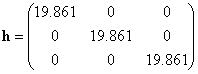
is used.
If the CHARMM package is not available, one can use "MPDyn_Prep"
instead. Before executing "MPDyn_Prep", a PSF file should be
generated by "PSFMaker".
"PSFMaker < Inputs/input_psf.data"
This generates a PSF file, "NaClw.psf". Then to convert the pdb
file, "Initial.pdb" to the crd file, "initial.crd",
"MPDyn_Prep" is used.
"MPDyn_Prep < Inputs/input_prep.data"
Now you should obtain two files, "initial.crd" and "NaClw.pdf".
- Condition file (Job script) : input.data
A sample for "input.data" is provided in the directory ./Inputs
as "input.MD". In this example, the system is modeled by the
CHARMM PARAM27 force field. Since all parameters used here are listed in
the default files (./param/top_charmm27.prm and ./param/par_charmm27.prm),
it is not required for users to make any changes in those parameter files.
Before starting an MD run, change the script filename to "input.data".
Then, to start an MD simulation, type
"MPDynS"
or for MPI parallel computing, for example,
"mpirun -np ** MPDynP"
This MD run will take about 6 minites on a single nodes of the Pentium
IV 3.0GHz machine.
Outputs
- In this example, the following two files will be generated.
(JOBName).moni: Thermodynamics quantity
(JOBName).r001: Trajectory
JOBName="TEST" in this sample.
Check your results
- This program package also provides an executable, "Eplot", to
convert the monitoring data, e.g., "TEST.moni", into a plotter-friendly
format. Gnuplot works with the resultant files. You should input some data
according to the messages shown during the interactive execution. For the
user's help, a sample input script, "input_eplot.data", is provided.
If you use it, type "Eplot < Inputs/input_eplot.data". Note
that you should make a directory, ./E_data, before executing Eplot. You
will find several data files in the directory.
If gnuplot is available in your computer, try to use it with "gnuplot
Inputs/ene.gnp". Then you will obtain some plots for energies, cell
dimension, etc.
- MPDyn also provides some tools for analyzing trajectory data. Here you
may find a file, input.analysis, in the directory ./Inputs. This is an
example of "input.data" (job script) for calculating the radial
distribution functions. To use it, change filename to input.data, then
execute MPDynS or MPDynP. In the case of "Analysis", the resultant
file are stored in the directory, ./Analy. Therefore, you should make the
directory before executing any "Analysis" with MPDynS.
Again, "gnuplot Inputs/gr.gnp", you will obtain sample plots.
NOTE: You will need more statistics to obtain an accurate RDF. Make sure
that this sample is just to show how this software works.
Top of this page
In this example, you will learn a way to treat a new molecule. DPhPC is
a molecule which has ether linkage instead of ordinary ester one between
the hydrophobic chains and the glycerol backbone. The parameters for the
ether group were determined by ab initio molecular orbital calculation,
which are already listed in the parameter file. However, a topology file
for the new molecule, DPhPC, is still required to perform this MD simulation.
All files needed in this tutorial are supplied in MPDyn/case_study/Membrane_MD/DPhPC.
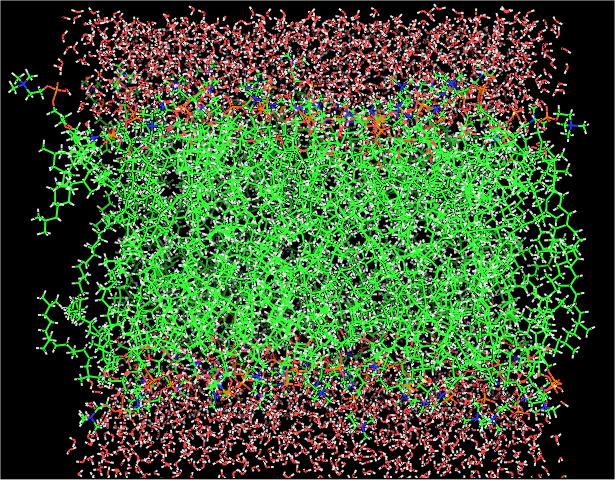
System
| DPhPC (lipid) |
72 |
| TIP3P (water) |
2088 |
Inputs
- Because diphytanoyl phosphatidylcholine (DPhPC) is not available in the
default CHARMM topology file, the first thing one should do is to make
a topology file for DPhPC. A sample file is "top_DPhPC.prm".
It is instructive to see the contents of this topology file. Detail description
for these files could be found in CHARMM development project. Then, you may make a PSF file, "DPhPCw.psf", with "PDFMaker
< Inputs/input_psf.data". In this sample, a configuration is supplied
as a binary file, "restart.dat".
- A sample job-script file is given as "Inputs/input.MD". After
changing the filename to "input.data", user may start this MD
simuation. The parameters given in the sample job-script are useful for
the parallel calculation with more than about 10 processors.
NOTE: In this software, the book-keeping method, which makes a list of
atomic pairs, is used to reduce the calculation of the interatomic interaction.
The optional flag, "MAXPAIR" in the keyword, "PBC",
which is described in the job-script file, "input.data", to declare
the maximum number of listed pairs, i.e., to maintain the memory space
for the pair list, should be larger than the actual number of the pairs.
In the case of large systems, this number becomes so large that the allocated
memory space for the pair list exceeds the physical memory size. In this
case, you will get a core dump, otherwise wait a long time to get a response
due to disk swap. To prevent from this, you should use a computer system
with sufficiently large memory or with distributed-memory multiple processors.
For the latter case, the number to be given to "MAXPAIR" is the
number of actual pairs devided by that of the processors. As a guide to
estimation, MAXPAIR=1.0-1.5million is the maximum number to be allowed
for 1Gb memory system.
Outputs
- You will have a couple of files, DPhPC_298K.moni and DPhPC_298K.r001. This
sample MD is not sufficiently long for the analysis.
Reference
- K. Shinoda et al., J. Chem. Phys. 121 9648 (2004).
Top of this page
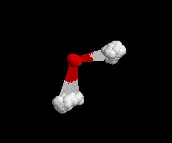
In this example, you will learn the way to use rigid-body approximation
in MD simulations.
All files needed in this tutorial are supplied in MPDyn/case_study/Water_MD/SPCE/.
System
Inputs
- Since the parameters for the SPC/E water has been already given in the
OPLS parameter file, the first thing to do is to prepare the configuration
file with the PDB format, in which each atom has the name corresponding
to that in the topology file. This file is given as "Initial.pdb".
Using a module, "ToolParam", user should make a file, "RigidBodyModel.prm",
where the atomic mass and the molecular structure defined in the body-fixed
frame. Note that "ToolParam" generates only a few samples, and
users should make the file, "RigidBodyModel.prm", for their own
purpose. "ToolParam" gives a resultant xyz files in the directory
./check, which should be made before executing this program. Then, type
"ToolParam < Inputs/input_bodyfixed.data". The file "RigidBodyModel.prm"
should be generated in the directory, ./param.
- Next, user should make a couple of files, "initial.crd" and "initialRB.dat". The former is the conventional CRD file, while the latter should contain the positions of the center of mass of each rigid-body and the Euler angles (quartenion). User can generate these files by "MPDyn_Prep". The Euler angles are calculated by fitting the given configuration to the body-fixed coordinates defined in "RigidBodyModel.prm". A sample input script for this program is provided as "./Inputs/input_prep.data". Just for your convenience, you can check a file "MSDcheck.dat", which will be generated in the current directory. This contains a list of the mean-square deviations (error) of the Euler-angles for each rigid-body due to this fitting procedure. Typical MSD is about 10-2Å2.
- Then you can start an MD run in the NVT ensemble with a job-script file
provided "./Inputs/input.NVT". After changing the filename to
"input.data", you can execute MPDyn for a 10ps-NVT-MD. In this
example, the system temperature is controlled by the velocity scaling algorithm
just to obtain a thermal equilibrium of the built system which may contain
a lot of unphysical contacts between atoms. After this calculation, therefore,
you will need to change the ensemble and algorithms. For this purpose,
"Xconverter" is useful. This executable read two script files,
"input.data" and "input_convert.data". The former should
be the same file, which generate the "restart.dat", whereas one
change is needed for the flag, STATUS. "RESTART" should be chosen
for this flag. The file, "input_convert.data", has the same format
as "input.data" but has slightly different keywords. A sample
file for "input_convert.data" is also provided in the directory
./Inputs. After executing "Xconverter", you should try an NPT-MD
run with the different sample job-script file, which is supplied as "Inputs/input.NPT".
Outputs
- For NVT-MD, you will obtain NVTMD.moni. For NPT-MD, NPTMD.moni and NPTMD.r001
will be generated. User should see if these simulations are finalized correctly
by checking the results.
Reference
- W. Shinoda and M. Mikami, J. Comput. Chem. 24 920 (2003).
Top of this page
In this example, you will learn how path integral MD works.
All files needed in this tutorial are supplied in MPDyn/case_study/Water_PIMD/SPCF/.
System
Inputs
- The procedure to conduct a path integral MD (PIMD) simulation is the same
as a classical MD. At first, "Initial.pdb" provided in the current
directory should be converted to "Initial.crd" by MPDyn_Prep.
A script file, ./Inputs/input_prep.data" will be useful. Then, using
"Inputs/input.data", a PIMD simulation in canonical ensemble
will be carried out. In this example, the heat capacity of the isolated
water is calculated. Note that the keyword, "HEATCAPACITY", is
valid only for the SPCF water system. Users who want to use this option
for different molecules should change the program source files to some
extent.
Outputs
- In addition to the ordinary output file, as a result of the choice of "HEATCAPACITY",
you will find a couple of files in the current directory. "Cv0.data"
contains accumulative averagies of several Cv. The data listed in one line are [ PIMD Step, CvT, CvV, CvCV,
CvDV, CvDCV ]. "Ene0.data" contains accumulative averagies of energy. The
data listed in one line are [ time step, ET, EV, ECV, <V> ].
In this example, the imaginary time slice P=16 is used, which is not large
enough to obtain a well converged results for Cv. User may try to use P=128 to obtain a correct answer. In addition, note
that this trial PIMD may be too short to see the convergence as for Cv. For more details, user should consult the following paper.
Reference
- W. Shinoda and M. Shiga, Phys. Rev. E 71 041204 (2005).
- M. Shiga and W. Shinoda, J. Chem. Phys. 123 134502(2005).
Top of this page
In this example, you will learn the way to conduct a DPD simulation.
All files needed are supplied in MPDyn/case_study/DPD/Water/.
Inputs
- In case of simple particle of DPD, if you do not have an initial configuration,
it will be automatically generated. A file which stores interaction parameters
for the conservative force, is necessary. The parameter file is assumed
as "./param/interaction.param" without specification in "input.data".
Users can try to use three job-script files provided in ./Inputs/.
Outputs
- You will find several files having (JOB_NAME) in the header of their filenames.
"(JOB_NAME).Ener" contains [ Time, Internal energy, Potential
energy, Kinetic energy ].
"(JOB_NAME).Temp" contains [ Time, Temperature, Translational
Temp., Rotational Temp. ]. The latter two are calculated only in the case
of colloidal particles.
"(JOB_NAME).MSD" contains [Time, mean-square displacements]
"(JOB_NAME).Pres" contains [Time, Pressure, Virial]
"(JOB_NAME).virial" contains [Time, Virial from the conservative
force, Virial from random force, Virial from dissipative force]
"(JOB_NAME).moni" contains some information of the simulation
conditions.
"(JOB_NAME).Average" contains averages of several thermodynamic
quantities.
"(JOB_NAME).gr" gives a radial distribution function. This file
is produced only for simple fluid (one component and single particle).
"(JOB_NAME).xyz" contains trajectory of the system. Now this
file is vacancy. This xyz file is useful, when you want to make an animation
of your DPD run. To produce this file, you should change the value of "COORD="
in the keyword "STEP_NUMBER" in "input.data".
NOTE: All quantities are given in the reduced unit. You will see that some
thermodynamic quantities depend on the choice of integrators.
Reference
- B. Hafskjold, C. C. Liew, and W. Shinoda, Mol. Simul. 30 879 (2004).
Top of this page
This is an example of the MD calculation of a solid SiO2. All files needed are given in MPDyn/case_study/SiO2/.
Inputs
- Here we use the BKS force field; van Beest et al., Phys. Rev. Lett. 64
1955 (1990). Topology and parameter files are given in param directory.
At first, to generate the initial configuration file, initial.crd, you
may use MPDyn_Prep with a input file, Inputs/input_prep.
- Then you may carry out an NPT-MD run using "input.data" supplied
in the param directory.
Outputs
- Data for some plots of energy and cell fluctuations will be obtained using
Eplot with Inputs/input_eplot.data. The directory, E_data, should be made
before Eplot conducted. You will get some examples by "gnuplot Inputs/ene.gnp".
Top of this page
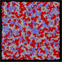
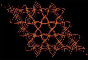
Initial random configuration |
 |
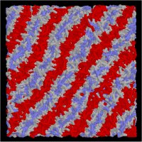
Lammelar |
Here we give a simple example for surfactant/water system to understand
how to treat the molecular system in DPD calculations. All files needed
are supplied in MPDyn/case_study/DPD/Surfactant/.
System
| Dimer (surfactant) |
2250 |
| W (water) |
1500 |
Inputs
- An initial configuration must be prepared manually for the molecular systems.
The filename for the initial configuration should be restartDP.dat. The
first N lines in the file should be coordinates and velocities; each line
denotes x, y, z, vx, vy, vz. The next (N+1)th line denotes the box displacement,
which is used only in case of sheared boundary (Lees-Edwards) and usually
should be 0.0. And the (N+2)th, last line is time, which is usually 0.0
for an intial configuration. E.g. see 'restartDP.dat'.
- A topology file should be given for each molecule having more than two
sites in the param/ directory with the file name of "{MOLNAME}Model.param".
In this example, a surfactant molecule called "Dimer" is used
and a file, "./param/DimerModel.param" is used to give topology
data.
- Interaction parameters should be provided in "./param/interaction.param".
Outputs
- Basically all output files are the same as those in Ex. 5. See initial.xyz
and final.xyz; initial and final snapshots of the simulated system. In
the file, atom name is automatically assigned arbitrary just to identify
the different particle types. Because the reduced unit is used, you may
have a problem in the visualization by a conventional molecular viewer.
Rescaling your coordinate often helps you to get it visualized.
Top of this page
Return to HOME